Tanveer Khan Data Scientist @ NextGen Invent | Research Scholar @ Jamia Millia Islamia
Market basket analysis using Apriori algorithm
Market basket analysis for finding association rules is a technique to identify underlying relations between different items. Take an example of a Super Market where customers can buy variety of items. Usually, there is a pattern in what the customers buy. For instance, mothers with babies buy baby products such as milk and diapers. Damsels may buy makeup items whereas bachelors may buy beers and chips etc. In short, transactions involve a pattern. More profit can be generated if the relationship between the items purchased in different transactions can be identified.
For instance, if item A and B are bought together more frequently then several measures can be taken to increase the profit. For example:
- A and B can be placed together so that when a customer buys one of the product he doesn't have to go far away to buy the other product.
- People who buy one of the products can be targeted through an advertisement campaign to buy the other.
- Collective discounts can be offered on these products if the customer buys both of them.
- Both A and B can be packaged and sold together.
The process of identifying an associations between products is called association rule mining.
Apriori Algorithm
Apriori is a popular algorithm for extracting frequent itemsets with applications in association rule learning. The apriori algorithm has been designed to operate on databases containing transactions, such as purchases by customers of a store. An itemset is considered as "frequent" if it meets a user-specified support threshold. For instance, if the support threshold is set to 0.5 (50%), a frequent itemset is defined as a set of items that occur together in at least 50% of all transactions in the database.
Concepts related to Apriori algorithm
Here we will discuss some general concepts related to the Apriori algorithm.
Support
Support refers to the default popularity of an item and can be calculated by finding number of transactions containing a
particular item divided by total number of transactions. Suppose we want to find support for item B. This can be calculated as:
Support(B) = (Transactions containing (B))/(Total Transactions)
Confidence
Confidence refers to the likelihood that an item B is also bought if item A is bought. It can be calculated by finding the number of
transactions where A and B are bought together, divided by total number of transactions where A is bought. Mathematically, it can be represented as:
Confidence(A→B) = (Transactions containing both (A and B))/(Transactions containing A)
Lift
Lift(A -> B) refers to the increase in the ratio of sale of B when A is sold. Lift(A –> B)
can be calculated by dividing Confidence(A -> B) divided by Support(B). Mathematically it can be represented as:
Lift(A→B) = (Confidence (A→B))/(Support (B))
Steps Involved in Apriori Algorithm
For large sets of data, there can be hundreds of items in hundreds of thousands transactions. The Apriori algorithm tries to extract rules for each possible combination of items. For instance, Lift can be calculated for (Item 1, Item 2);, (Item 1, Item 3);, (Item 1, Item 4);, and then (Item 2, Item 3);, (Item 2, Item 4);, and then combinations of items e.g. (Item 1, Item 2, Item 3); similarly (Item 1, Item2, Item 4);, and so on.
As you can see from the above example, this process can be extremely slow due to the number of combinations. To speed up the process, we need to perform the following steps:
- Step 1: Set a minimum value for support and confidence. This means that we are only interested in finding rules for the items that have certain default existence (e.g. support) and have a minimum value for co-occurrence with other items (e.g. confidence).
- Step 2: Extract all the subsets having higher value of support than minimum threshold.
- Step 3: Select all the rules from the subsets with confidence value higher than minimum threshold.
- Step 4: Order the rules by descending order of Lift.
Implementation of Apriori Algorithm in Python
In this section we will use the Apriori algorithm to find rules that describe associations between different products given 7500 transactions over the course of a week at a American retail store. The dataset can be downloaded from here .
Import packages
The first step, as always, is to import the required packages. Execute the following script to do so:
   # import packages
   import pandas as pd
   from mlxtend.frequent_patterns import apriori
   from mlxtend.frequent_patterns import association_rules
Reading the Dataset
Now let's load the dataset into the working directory and see what we're working with.
  # Read the gorcery data
  items_data= pd.read_csv("./Grocery_data.csv",header=None)
Let's call the head() function to see how the dataset looks:
print("Dataset:", items_data.head(15),"\n")
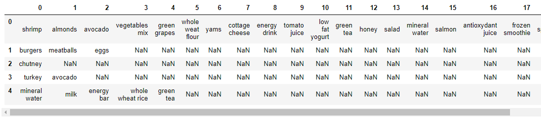
A snippet of the dataset is shown in the above figure. If we carefully examine the data, we can see that there is no header in this datset. Each row corresponds to a transaction and each column corresponds to an item (s) purchased in that specific transaction. The NaN tells us that the item represented by the column was not purchased in that specific transaction.
In this dataset there is no header row. But by default, pd.read_csv function treats first row as header. For this, we have added "header=None" option to pd.read_csv function, as shown above in the reading the data code snippet.
Data Pre-Processing
The Apriori module from "mlxtend" package we are going to use requires our dataset to be in the one-hot encoded form i.e in the form of "0" or "1". Currently we have our data in the form of a pandas dataframe. To convert our pandas dataframe to one-hot encoded dataframe, execute the following script:
# one hot encoding for supplying data in the apriori algorithm
for i, rows in items_data.iterrows():
  labels={}
  uncommons=list( set(unique_items)-set(rows))
  commons=list( set(unique_items).intersection(rows))
  for un in uncommons:
    labels[un] = 0
  for com in commons:
    labels[com] = 1
  encoded_vals.append(labels)

# create a dtaframe for enocoded data
encoded_data = pd.DataFrame(encoded_vals)
print("\nOne hot encoded data:\n", encoded_data.head(10),"\n")
Applying Apriori
The next step is to apply the Apriori algorithm on the dataset. To do so, we can use the apriori class that we imported from the mlxtend library
The apriori class requires some parameter values to work. The first parameter is the one-hot encoded dataframe that we want to extract rules from. The second parameter is the min_support parameter. This parameter is used to select the items with support values greater than the value specified by the parameter. Next, the use_colnames parameter that If True, uses the DataFrames' column names in the returned DataFrame instead of column indices. Other parameter max_len takes the value for maximum length of the itemsets generated. Finally, the verbose parameter shows the number of iterations. Executing the following script we can have our frequent itemsets generated:
frequent_items = apriori(encoded_data, min_support=0.0085, use_colnames=True, verbose=1)
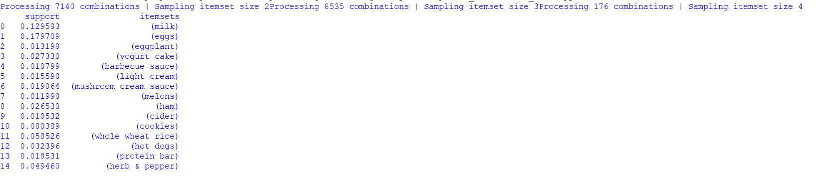
Here, we will print the top 15 frequent itemsets generated susing apriori algorithm.
print("Top 15 frequent items:\n",frequent_items.head(15),"\n")
Figure below shows the frequent itemsets with their support values.
For generating the association rules for the itemsets generated using apriori algorithm we will use the 'association_rules' class from the "mlxtend" package. The association_rules class takes 'frequent_ itemsets' dataframe, 'metrics' and 'min threshold' values as some parameters. Executing the following script for generating the association rules:
association_rule_generated_confidence= association_rules(frequent_items, metric="confidence", min_threshold=0.25)
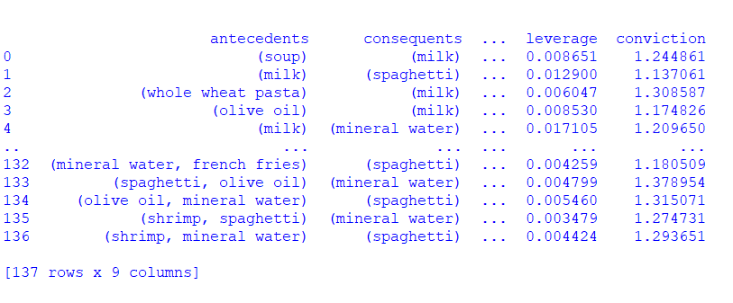
Here, we will print the association_rules generated using "confidence" as a metric with 0.25 as a threshold value.
print("association rules generated through confidence metrics:\n", association_rule_generated_confidence.head(15),"\n")
Figure below shows the association rules generated with lift, confidence, leverage, and support values.
Conclusion
Association rule mining algorithms such as Apriori are very useful for finding associations between our data items. They are easy to implement and have high generalizability.
However Appriori algorithm suffer from issues like, the size of itemset from candidate generation could be extremely large and lots of time gets wasted on counting the support since we have to scan the itemset database over and over again till the algorithm converges.
References
- Ilayaraja, M., & Meyyappan, T. (2013, February). Mining medical data to identify frequent diseases using Apriori algorithm. In 2013 International Conference on Pattern Recognition, Informatics and Mobile Engineering (pp. 194-199). IEEE.
- Kaur, M., & Kang, S. (2016). Market Basket Analysis: Identify the changing trends of market data using association rule mining. Procedia computer science, 85, 78-85.
- apriori-python. (2020). Retrieved 23 August 2020, from https://pypi.org/project/apriori-python