Tanveer Khan Data Scientist @ NextGen Invent | Research Scholar @ Jamia Millia Islamia
Electroencephalography (EEG) based subject identification
1. Introduction
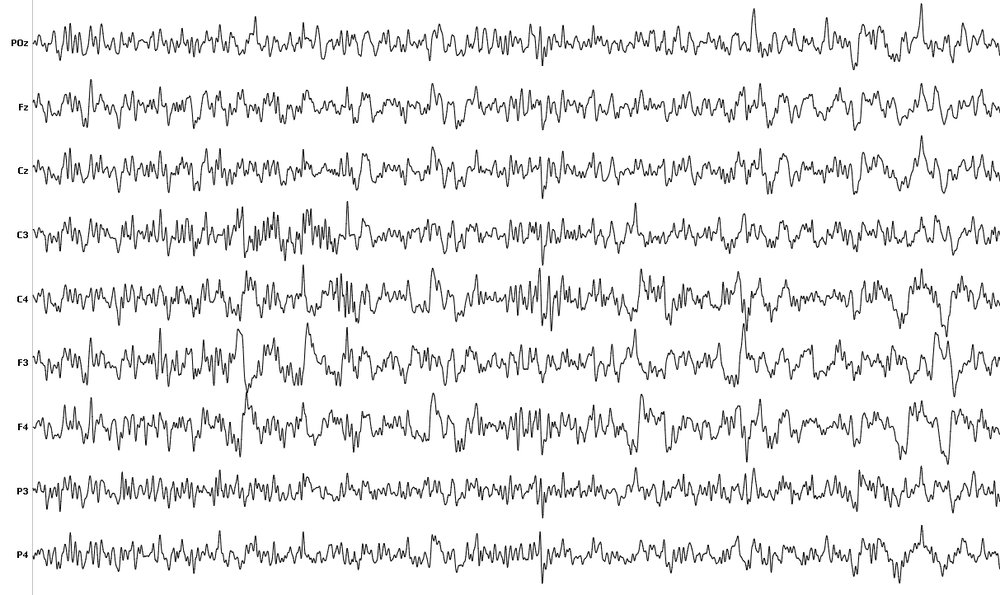
EEG is a non-invasive brain imaging technique that measures difference in electrical voltage (micro-voltage), that occur as a part of neural activity in the human brain. EEG signal data acquired from subjects are unique for every individual and offers stability in signal patterns that are needed in designing biometric systems and thus have been explored as a potential biometric trait.
A biometric system can perform either identification or authentication task. In identification, biometric system establishes the identity of the user i.e. it has a one-to-many (1: N) relationship while in authentication a biometric system verifies the claimed identity of the user (1:1) by matching the given sample with the stored template in the database. Here, we will perfrom identification of subjects' using publicly available dataset having EEG recordings from 48 subjects.
2. About Dataset
STEW-SI dataset consists of raw EEG data from 48 subjects who participated in a multitasking workload experiment utilizing the SIMKAP multitasking test. The subjects’ brain activity at rest was also recorded before the test and is included as well. The Emotiv EPOC device, with sampling frequency of 128Hz and 14 channels was used to obtain the data, with 2.5 minutes of EEG recording for each case. Subjects were also asked to rate their perceived mental workload after each stage on a rating scale of 1 to 9 and the ratings are provided in a separate file.
3. Methodology
Typical EEG subject identification pipeline includes tasks such as: signal-acquisition, signal pre-processing, features extraction, and classification phase.
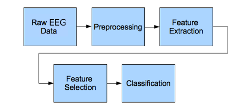
Figure 1. EEG signal processing steps
Here, our EEG data is already in acquired form so, we can start from the next phase in the pipeline which is the signal pre-processing phase.
3.1 Signal pre-processing
Here we will filter our EEG dataset to remove noise and artifacts. For this purpose, we will use butterworth filter.
Importing packages
  import pandas as pd
  import numpy as np
  from numpy import mean
  from numpy import std
  import matplotlib.pyplot as plt
  import scipy.io
  import scipy.signal
  from scipy.signal import butter,filtfilt,find_peaks,find_peaks, resample
  from scipy import stats
  from scipy.stats import skew, kurtosis
  from sklearn import preprocessing
  from sklearn.model_selection import train_test_split
  from sklearn.metrics import classification_report,confusion_matrix,accuracy_score
  from sklearn.metrics import roc_curve,auc, precision_score,recall_score,f1_score
  from sklearn.feature_selection import SelectKBest, chi2
  from sklearn.ensemble import ExtraTreesClassifier
  from keras import layers, models, regularizers
  import mne
  from mne import find_events, fit_dipole
  from autoreject import AutoReject
  import seaborn as sns
  import sys
  import statistics as st
  from keras.utils import to_categorical
  #import pywt
  import sys
  import antropy as an
  import time
  Channels = ["AF3", "F7", "F3", "FC5", "T7", "P7", "O1", "O2", "P8", "T8", "FC6", "F4", "F8", "AF4"]

  ##1.1 Filter requirements.
  T =     150         # Sample Period,    Seconds
  fs =    128         # Sample rate,      Hz
  cutoff = 40          # Desired cutoff frequency of the filter, Hz
  nyq = 0.5 * fs      # Nyquist Frequency
  order = 1           # sin wave can be approx represented as quadratic
  n = int(T * fs)+1   # Total number of samples

  t=np.linspace(0,150,19200)

  normal_cutoff = [3/nyq ,40/nyq]
  b, a = butter(order, normal_cutoff, btype='bandpass', analog=False)    # Get the filter coefficients
  SS=0
  TIMES = np.zeros([48])
3.2 Feature extraction
From the pre-processed EEG signal 17 features which included statistical, entropy, and energy features were extracted.
  Features = ["mean_PSD",         "STD_PSD",
              "A_mean",           "A_STD",            "A_Var",
              "A_range",          "A_skew",           "A_kurtosis",
              "Permutation_E",    "Spectral_E",       "SVD_E",
              "Approximate_E",    "Sample_E",         "Petrosian_FD",
              "Katz_FD",          "Higuchi_FD",
              "Detrended fluctuation analysis",
              "Label"]
                                # Features' Names
  Features_df = pd.DataFrame(columns = Features)    # Features of Subject 1

  # Read Data
start_time = time.time()
for s in range(1,49):
    if s < 10:
        URL=".\\STEW Dataset\\sub0"+str(s)+"_hi.txt"
    else:
        URL=".\\STEW Dataset\\sub"+str(s)+"_hi.txt"

    Data = pd.read_csv(URL, sep="  ", header=None)
    Data.columns=Channels
    print("Extracting Features From Subject: ",s)
    print("--- %s seconds ---" % (time.time() - start_time))
    TIMES[s-1] = time.time() - start_time

    for Ch in Channels:
        # Pre-Processing
        Data.insert(0, ''.join([Ch + " Filtered"]), filtfilt(b,a,Data[Ch]))
        Data = Data.drop(Ch, axis=1)
        Data.insert(0, ''.join([Ch + " Despiked"]), Data[''.join([Ch + " Filtered"])].where(Data[''.join([Ch + " Filtered"])] < Data[''.join([Ch + " Filtered"])].quantile(0.97), Data[''.join([Ch + " Filtered"])].mean()))
        Data = Data.drop(''.join([Ch + " Filtered"]), axis=1)
        Data.insert(0, Ch, Data[''.join([Ch + " Despiked"])].where(Data[''.join([Ch + " Despiked"])] > Data[''.join([Ch + " Despiked"])].quantile(0.05), Data[''.join([Ch + " Despiked"])].mean()))
        Data = Data.drop(''.join([Ch + " Despiked"]), axis=1)
    w=0
    for window in range(0,60):
        EEG_Window = Data[w:w+640] # Windowing, Window Len: 5 Sec, Overlap: 2.5 Sec
        w=w+320
        Fet = np.zeros([300]) #Temporal Features + Lable array
        Fet_ch = np.zeros([18])
        i=0
        for i in range(14):
            channel = EEG_Window[Channels[i]]
            # Feature Extraction


            # PSD Features
            f, Pxx =scipy.signal.welch(channel,fs) #Extract PSD according to Welch thiorem

            Fet[i]         = mean(Pxx)                                                      # Mean of PSD

            Fet[i+14]       = std(Pxx)                                                      # Standered Deviation of PSD

            # Statistics Features
            Fet[i+28]      = mean(channel)                                                  # Amplitude Mean

            Fet[i+42]      = std(channel)                                                   # Amplitude Standered Deviation

            Fet[i+56]      = np.var(channel)                                                # Amplitude variance

            Fet[i+70]      = max(channel)-min(channel)                                      # Amplitude Range

            Fet[i+84]      = skew(channel)                                                  # Amplitude Skew

            Fet[i+98]      = kurtosis(channel)                                              # Amplitude kurtosis

            # Entropy Features
            Fet[i+112]      = an.perm_entropy(channel, order=3, normalize=True)                 # Permutation entropy

            Fet[i+126]      = an.spectral_entropy(channel, 100, method='welch', normalize=True) # Spectral entropy

            Fet[i+140]      = an.svd_entropy(channel, order=3, delay=1, normalize=True)         # Singular value decomposition entropy

            Fet[i+154]      = an.app_entropy(channel, order=2, metric='chebyshev')              # Approximate entropy

            Fet[i+168]      = an.sample_entropy(channel, order=2, metric='chebyshev')           # Sample entropy

            # Fractal dimension Features
            Fet[i+182]      = an.petrosian_fd(channel)                                          # Petrosian fractal dimension

            Fet[i+196]      = an.katz_fd(channel)                                               # Katz fractal dimension

            Fet[i+210]      = an.higuchi_fd(channel, kmax=10)                                   # Higuchi fractal dimension

            Fet[i+224]      = an.detrended_fluctuation(channel)                                 # Detrended fluctuation analysis

        Fet_ch[0]      = mean(Fet[0:14])        # Mean of PSD
        Fet_ch[1]      = mean(Fet[14:28])       # Standered Deviation of PSD
        Fet_ch[2]      = mean(Fet[28:42])       # Amplitude Mean
        Fet_ch[3]      = mean(Fet[42:56])       # Amplitude Standered Deviation
        Fet_ch[4]      = mean(Fet[56:70])       # Amplitude variance
        Fet_ch[5]      = mean(Fet[70:84])       # Amplitude Range
        Fet_ch[6]      = mean(Fet[84:98])       # Amplitude Skew
        Fet_ch[7]      = mean(Fet[98:112])      # Amplitude kurtosis
        Fet_ch[8]      = mean(Fet[112:126])     # Permutation entropy
        Fet_ch[9]      = mean(Fet[126:140])     # Spectral entropy
        Fet_ch[10]     = mean(Fet[140:154])     # Singular value decomposition entropy
        Fet_ch[11]     = mean(Fet[154:168])     # Approximate entropy
        Fet_ch[12]     = mean(Fet[168:182])     # Sample entropy
        Fet_ch[13]     = mean(Fet[182:196])     # Petrosian fractal dimension
        Fet_ch[14]     = mean(Fet[196:210])     # Katz fractal dimension
        Fet_ch[15]     = mean(Fet[210:224])     # Higuchi fractal dimension
        Fet_ch[16]     = mean(Fet[224:238])     # Detrended fluctuation analysis
        Fet_ch[17]     = s-1

        Features_df.loc[SS]=Fet_ch
        SS=SS+1
Features_df.to_csv('extractedFeatures.csv')
print("All features were extracted and saved")
Figure below shows the features map for the subject identification task.
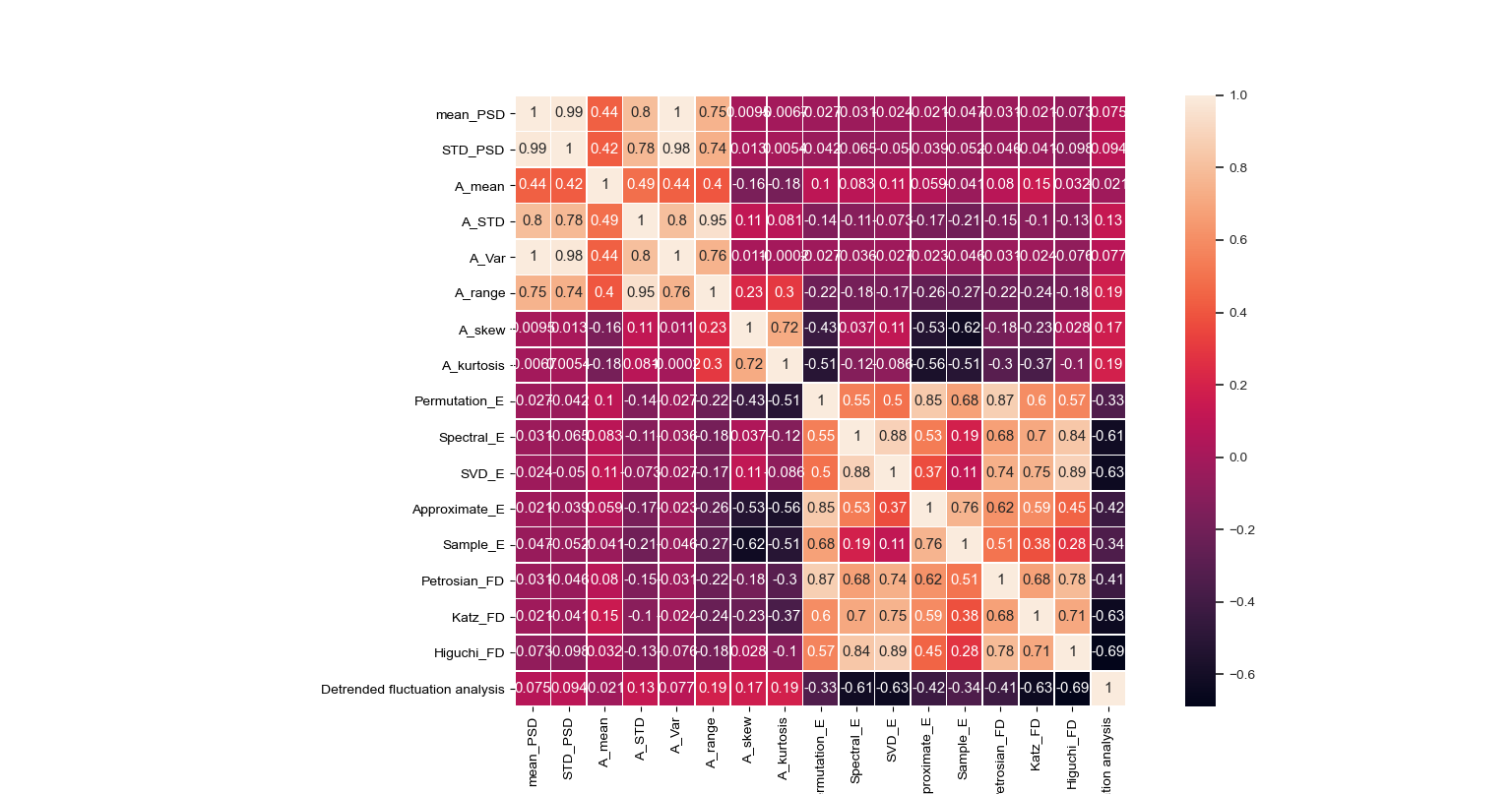
Figure 2. Features Map.
3.3 Classification of subjects
For supplying data to the neural network model, we will label our data. Furthermore, we will split our labelled dataset into train, test, and validation sets.
  ## Shuffling
  Data = Features_df.sample(frac = 1)
  features = Data[[x for x in Data.columns if x not in ["Label"]]]   # Data for training
  Labels = Data['Label']                                            # Labels for training
  Labels = Labels.astype('category')

  # Prepare Train and test Data
  splitRatio = 0.3
  train, test = train_test_split(Data ,test_size=splitRatio,
                               random_state = 123, shuffle = True)  # Spilt to training and testing data

   train_X = train[[x for x in train.columns if x not in ["Label"]]]   # Data for training
   train_Y = train['Label']                                            # Labels for training

   ###4.5.2 Testing Data
   test_X = test[[x for x in test.columns if x not in ["Label"]]]     # Data fo testing
   test_Y = test["Label"]                                              # Labels for training

   ###4.5.3 Validation Data
   x_val = train_X[:200]                                                # 50 Sample for Validation
   partial_x_train = train_X[200:]
   partial_x_train = partial_x_train.values

   y_val = train_Y[:200]
   y_val = to_categorical(y_val)
   partial_y_train = train_Y[200:]
   partial_y_train = partial_y_train.values
   partial_y_train = to_categorical(partial_y_train)

   print("Data is prepeared")
3.3.1 Building our Neural network classification model
For performing the identification task Artificial neural network (ANN) was used.
  # Classification Model

  ## Building Model

  ### Architecture
  model = models.Sequential()
  model.add(layers.Dense(200, activation = 'relu', input_shape=(17,),kernel_regularizer=regularizers.l1(0.01)))
  #model.add(layers.Dropout(0.3))
  model.add(layers.Dense(150, activation = 'relu'))
  model.add(layers.Dense(100, activation = 'relu'))
  #model.add(layers.Dropout(0.3))
  model.add(layers.Dense(75, activation = 'relu'))
  model.add(layers.Dense(48,  activation= 'softmax'))

  ### Hyper Parameters Tuning
  model.compile(optimizer='Adam',
                loss='categorical_crossentropy',
                metrics=['accuracy'])

  print("Classifier Bulit\n")
  print("Start Training\n")

  ## Training Model
  history = model.fit(partial_x_train,
                      partial_y_train,
                      epochs = 5,                # initial value = 1000
                      batch_size = 16,              # initial value = 16
                      validation_data=(x_val, y_val))

  weights = model.get_weights()
  configs = model.get_config()

  Featuers_weights = np.apply_along_axis(mean, 1, weights[0])
  print("Finish Training")
3.3.2 Model Evaluation
Here, we will evaluate our build NN model performance in terms of training-validation accuracy and train-validation loss.
  ## Network Architecture
  print(model.summary())
  print("Start Evaluating Data")

  ## Training Process
  history_dict = history.history
  loss_values = history_dict['loss']
  val_loss_values = history_dict['val_loss']

  epochs = range(1,len(loss_values)+1)
  plt.figure()
  plt.plot(epochs, loss_values, 'bo', label="training loss", color='r')
  plt.plot(epochs, val_loss_values, 'b', label="validation loss")
  plt.title("Training and Validation Loss")
  plt.xlabel("Epoches")
  plt.ylabel("loss")
  plt.legend()
  plt.show()

  acc_values = history_dict['accuracy']
  val_acc_values = history_dict['val_accuracy']
  plt.figure()
  plt.plot(epochs, acc_values, 'bo', label="training acc", color = 'r')
  plt.plot(epochs, val_acc_values, 'b', label="validation acc")
  plt.title("Training and Validation acc")
  plt.xlabel("Epoches")
  plt.ylabel("acc")
  plt.legend()
  plt.show()
Figures below shows the training-validation loss and training-validation accuracy curves.
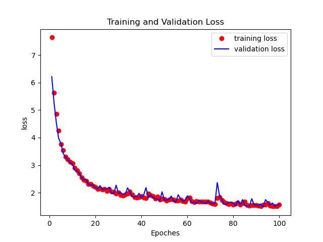
Figure 3. Training-validation loss curve.
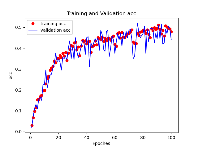
Figure 4. Training-validation accuracy curve.
3.3.3 Neural Network model evaluation on test data
Evaluating our NN model on test data and making predictions.
# Model Evaluation on Test data
## Prediction
ANN_predictions = model.predict(test_X)

Pred = np.zeros([len(ANN_predictions)])
for i in range(0,len(ANN_predictions)):
    Pred[i] = list(ANN_predictions[i]).index(max(ANN_predictions[i]))
ANN_Pred = pd.Series(Pred)
3.3.4 Results
For the evaluation of the performance of our NN classification model we will use standard metrics and plot the confusion matrix for the same.
  #### Metrics
  print("Accuracy:",accuracy_score(test_Y, ANN_Pred))
  print("f1 score:", f1_score(test_Y, ANN_Pred,average="micro"))
  print("precision score:", precision_score(test_Y, ANN_Pred,average="micro"))
  print("recall score:", recall_score(test_Y, ANN_Pred,average="micro"))
  print("confusion matrix:\n",confusion_matrix(test_Y, ANN_Pred))
  print("classification report:\n", classification_report(test_Y, ANN_Pred))

  #### Plots

  # plot Confusion Matrix as heat map
  plt.figure(figsize=(3,2))
  sns.heatmap(confusion_matrix(test_Y, ANN_Pred),annot=True,fmt = "d",linecolor="k",linewidths=3)
  plt.title("CONFUSION MATRIX",fontsize=20)
  plt.show()
Figure below shows the confusion matrix for the subject identification task.
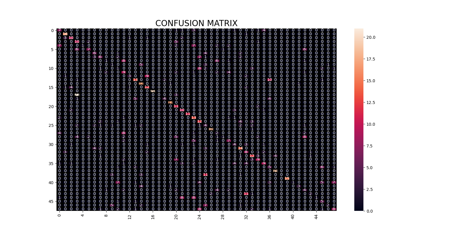
Figure 5. Confusion matrix for the subject identification task.
4. Conclusion
In this article, we build and tested our Neural Network model for the subject identification task on EEG data from 48 subjects. Our proposed model achieved an accuracy of 54% in correctly predicting subjects’ identity using their brain signals. Less accuracy may be attributed to the fewer data present for training and testing purpose.
Complete code can be found here.
References
- Khan, T. A., & Jabin, S. (2021). Recent trends in electroencephalography based biometric systems. In Recent Trends in Communication and Electronics (pp. 467-472). CRC Press.
- Wei Lun Lim, Olga Sourina, Lipo Wang, July 10, 2018, "STEW: Simultaneous Task EEG Workload Dataset", IEEE Dataport, doi: https://dx.doi.org/10.21227/44r8-ya50.