Gene Expression Classification

gene

1. Introduction

In this Article we will examine a small gene expression dataset, attempting to classify leukemia patients into one of two classes. We will use some machine learning models to perform the molecular classification of cancer.

2. Dataset

This dataset comes from a proof-of-concept study published in 1999 by Golub et al. It showed how new cases of cancer could be classified by gene expression monitoring (via DNA microarray) and thereby provided a general approach for identifying new cancer classes and assigning tumors to known classes. These data were used to classify patients with acute myeloid leukemia (AML) and acute lymphoblastic leukemia (ALL).

There are two datasets containing the initial (training, 38 samples) and independent (test, 34 samples) datasets used in the paper. These datasets contain measurements corresponding to ALL and AML samples from Bone Marrow and Peripheral Blood. Intensity values have been re-scaled such that overall intensities for each chip are equivalent.

3. Data Preparation


# Import all the libraries that we shall be using
import numpy as np
import pandas as pd

import matplotlib.pyplot as plt
import seaborn as sns
from mpl_toolkits.mplot3d import Axes3D
%matplotlib inline

from sklearn.preprocessing import StandardScaler
from sklearn.decomposition import PCA
from sklearn.model_selection import GridSearchCV, cross_val_score
from sklearn.metrics import accuracy_score, confusion_matrix
from sklearn.cluster import KMeans
from sklearn.svm import SVC
from sklearn.linear_model import LogisticRegression
from sklearn.naive_bayes import GaussianNB
from sklearn.ensemble import RandomForestClassifier


from keras.models import Sequential
from keras.layers import Dense
from keras.callbacks import EarlyStopping

Let's start by taking a look at our target, the ALL/AML label.


# Import labels (for the whole dataset, both training and testing)
y = pd.read_csv('../input/actual.csv')
print(y.shape)
y.head()

Output: (72, 2)

	patient	cancer
0	1	ALL
1	2	ALL
2	3	ALL
3	4	ALL
4	5	ALL

In the combined training and testing sets there are 72 patients, each of whom are labelled either "ALL" or "AML" depending on the type of leukemia they have. Here's the breakdown:


y['cancer'].value_counts()

Output:
ALL    47
AML    25
Name: cancer, dtype: int64

We actually need our labels to be numeric, so let's just do that now.


# Recode label to numeric
y = y.replace({'ALL':0,'AML':1})
labels = ['ALL', 'AML'] # for plotting convenience later on

Now we move on to the features, which are provided for the training and testing datasets separately.


# Import training data
df_train = pd.read_csv('../input/data_set_ALL_AML_train.csv')
print(df_train.shape)

# Import testing data
df_test = pd.read_csv('../input/data_set_ALL_AML_independent.csv')
print(df_test.shape)

Output:
(7129, 78)
(7129, 70)

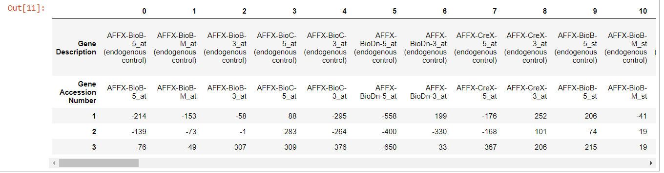
The 7129 gene descriptions are provided as the rows and the values for each patient as the columns. This will clearly require some tidying up.

Our first decision is: What should we do about all the "call" columns, one for each patient. No explanation for these is provided, so it's difficult to know whether they might be useful or not. We have taken the decision to simply remove them, but this may possibly not be the best approach.


# Transform all the call values to numbers (not used in this version)
# df_train.replace(['A','P','M'],['1','2','3'], inplace=True)
# df_test.replace(['A','P','M'],['1','2','3'], inplace=True)

# Remove "call" columns from training and testing data
train_to_keep = [col for col in df_train.columns if "call" not in col]
test_to_keep = [col for col in df_test.columns if "call" not in col]

X_train_tr = df_train[train_to_keep]
X_test_tr = df_test[test_to_keep]

Neither the training and testing column names are not in numeric order, so it's important that we reorder these at some point, so that the labels will line up with the corresponding data.


train_columns_titles = ['Gene Description', 'Gene Accession Number', '1', '2', '3', '4', '5', '6', '7', '8', '9', '10',
       '11', '12', '13', '14', '15', '16', '17', '18', '19', '20', '21', '22', '23', '24', '25', 
       '26', '27', '28', '29', '30', '31', '32', '33', '34', '35', '36', '37', '38']

X_train_tr = X_train_tr.reindex(columns=train_columns_titles)

test_columns_titles = ['Gene Description', 'Gene Accession Number','39', '40', '41', '42', '43', '44', '45', '46',
       '47', '48', '49', '50', '51', '52', '53',  '54', '55', '56', '57', '58', '59',
       '60', '61', '62', '63', '64', '65', '66', '67', '68', '69', '70', '71', '72']

X_test_tr = X_test_tr.reindex(columns=test_columns_titles)

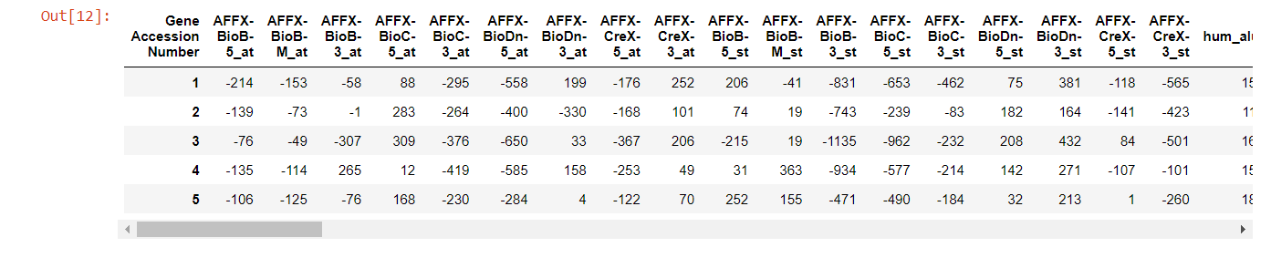
Now we can simply transpose the columns and rows so that genes become features and each patient's observations occupies a single row.


X_train = X_train_tr.T
X_test = X_test_tr.T

print(X_train.shape) 
X_train.head()

Output:
(40, 7129)

genedf

This is still messy as the first two rows are more or less duplicates of one another and we haven't yet created the column names. Let's simply turn the second row into the column names and delete the first row.


# Clean up the column names for training and testing data
X_train.columns = X_train.iloc[1]
X_train = X_train.drop(["Gene Description", "Gene Accession Number"]).apply(pd.to_numeric)

# Clean up the column names for Testing data
X_test.columns = X_test.iloc[1]
X_test = X_test.drop(["Gene Description", "Gene Accession Number"]).apply(pd.to_numeric)

print(X_train.shape)
print(X_test.shape)
X_train.head()

Output:
(38, 7129)
(34, 7129)

genedf1

That looks much better. We have the 38 patients as rows in the training set, and the other 34 as rows in the testing set. Each of those datasets has 7129 gene expression features.

But we haven't yet associated the target labels with the right patients. You will recall that all the labels are all stored in a single dataframe. Let's split the data so that the patients and labels match up across the training and testing dataframes.


# Split into train and test (we first need to reset the index as the indexes of two dataframes need to be the same before you combine them).

# Subset the first 38 patient's cancer types
X_train = X_train.reset_index(drop=True)
y_train = y[y.patient <= 38].reset_index(drop=True)

# Subset the rest for testing
X_test = X_test.reset_index(drop=True)
y_test = y[y.patient > 38].reset_index(drop=True)

Machine learning models work much better with data that's on the same scale, so let's create a scaled version of the dataset.


# Convert from integer to float
X_train_fl = X_train.astype(float, 64)
X_test_fl = X_test.astype(float, 64)

# Apply the same scaling to both datasets
scaler = StandardScaler()
X_train_scl = scaler.fit_transform(X_train_fl)
X_test_scl = scaler.transform(X_test_fl) # note that we transform rather than fit_transform

With 7129 features, it's also worth considering whether we might be able to reduce the dimensionality of the dataset. Once very common approach to this is principal components analysis (PCA). Let's start by leaving the number of desired components as an open question:


pca = PCA()
pca.fit_transform(X_train)


Output:
array([[-4.12032149e+03,  8.43574289e+03, -1.39441668e+04, ...,
         2.51106855e+03,  3.92187680e+03,  1.22642865e-11],
       [ 1.86283598e+04,  1.44078238e+04,  1.66177453e+04, ...,
        -2.30960132e+02, -1.04099055e+03,  1.22642865e-11],
       [-1.58238732e+04,  1.40484268e+04,  4.73320627e+04, ...,
         5.48675197e+02, -2.26227734e+03,  1.22642865e-11],
       ...,
       [ 6.50848905e+04, -5.49595793e+04,  1.67854688e+04, ...,
         1.18708820e+01, -1.47894896e+03,  1.22642865e-11],
       [ 4.97670530e+04, -3.81956823e+04,  2.93511865e+03, ...,
         2.66462156e+03,  7.99461277e+02,  1.22642865e-11],
       [ 1.08241948e+04, -1.68550421e+04, -9.46017931e+02, ...,
        -2.04773331e+03, -1.96917341e+03,  1.22642865e-11]])

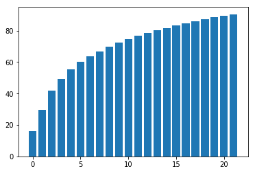
Let's set a threshold for explained variance of 90% and see how many features are required to meet that threshold.


total = sum(pca.explained_variance_)
k = 0
current_variance = 0
while current_variance/total < 0.90:
    current_variance += pca.explained_variance_[k]
    k = k + 1
    
print(k, " features explain around 90% of the variance. From 7129 features to ", k, ", not too bad.", sep='')

pca = PCA(n_components=k)
X_train.pca = pca.fit(X_train)
X_train_pca = pca.transform(X_train)
X_test_pca = pca.transform(X_test)

var_exp = pca.explained_variance_ratio_.cumsum()
var_exp = var_exp*100
plt.bar(range(k), var_exp);

22 features explain around 90% of the variance. From 7129 features to 22, not too bad.

pcagene

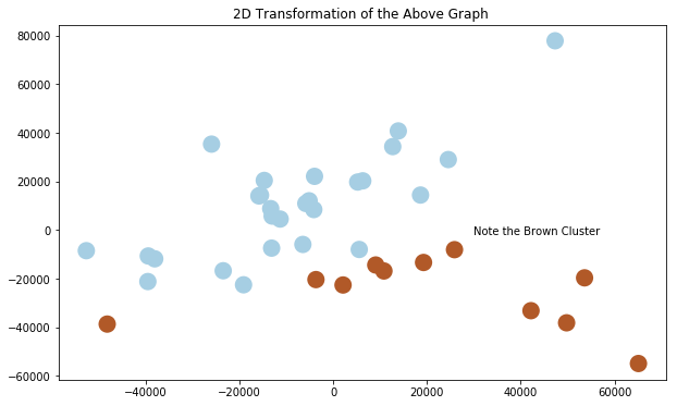
We can't plot something in 22 dimensions, so let's just see what the PCA looks like when we just pick the top three compoments.


pca3 = PCA(n_components=3).fit(X_train)
X_train_reduced = pca3.transform(X_train)

plt.clf()
fig = plt.figure(1, figsize=(10,6 ))
ax = Axes3D(fig, elev=-150, azim=110,)
ax.scatter(X_train_reduced[:, 0], X_train_reduced[:, 1], X_train_reduced[:, 2], c = y_train.iloc[:,1], cmap = plt.cm.Paired, linewidths=10)
ax.set_title("First three PCA directions")
ax.set_xlabel("1st eigenvector")
ax.w_xaxis.set_ticklabels([])
ax.set_ylabel("2nd eigenvector")
ax.w_yaxis.set_ticklabels([])
ax.set_zlabel("3rd eigenvector")
ax.w_zaxis.set_ticklabels([])

pcagene3d


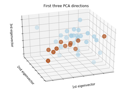
fig = plt.figure(1, figsize = (10, 6))
plt.scatter(X_train_reduced[:, 0],  X_train_reduced[:, 1], c = y_train.iloc[:,1], cmap = plt.cm.Paired, linewidths=10)
plt.annotate('Note the Brown Cluster', xy = (30000,-2000))
plt.title("2D Transformation of the Above Graph ")

scattergene

4. Model Building

4.1 Baseline

Let's start by establishing a naive baseline. This doesn't require a model, we are just taking the proportion of tests that belong to the majority class as a baseline. In other words, let's see what happens if we were to predict that every patient belongs to the "ALL" class.

Having prepared the dataset, it's now finally time to try out some models.


print("Simply predicting everything as acute lymphoblastic leukemia (ALL) results in an accuracy of ", round(1 - np.mean(y_test.iloc[:,1]), 3), ".", sep = '')

Output:
Simply predicting everything as acute lymphoblastic leukemia (ALL) results in an accuracy of 0.588.

4.2 K-Means Clustering

First we shall try an unsupervised clustering approach using the scaled data.


kmeans = KMeans(n_clusters=2, random_state=0).fit(X_train_scl)
km_pred = kmeans.predict(X_test_scl)

print('K-means accuracy:', round(accuracy_score(y_test.iloc[:,1], km_pred), 3))

cm_km = confusion_matrix(y_test.iloc[:,1], km_pred)

ax = plt.subplot()
sns.heatmap(cm_km, annot=True, ax = ax, fmt='g', cmap='Greens') 

# labels, title and ticks
ax.set_xlabel('Predicted labels')
ax.set_ylabel('True labels') 
ax.set_title('K-means Confusion Matrix') 
ax.xaxis.set_ticklabels(labels) 
ax.yaxis.set_ticklabels(labels, rotation=360);

Output:
K-means accuracy: 0.765

kmeanscm

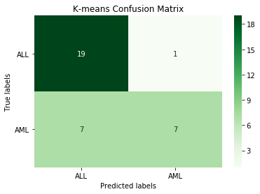
This K-means approach is better than the baseline, but we should be able to do better with some kind of supervised learning model.

4.3 Naive Bayes

For our first supervised model, we shall use a very straightforward naive bayes approach.


# Create a Gaussian classifier
nb_model = GaussianNB()

nb_model.fit(X_train, y_train.iloc[:,1])

nb_pred = nb_model.predict(X_test)

print('Naive Bayes accuracy:', round(accuracy_score(y_test.iloc[:,1], nb_pred), 3))

cm_nb =  confusion_matrix(y_test.iloc[:,1], nb_pred)

ax = plt.subplot()
sns.heatmap(cm_nb, annot=True, ax = ax, fmt='g', cmap='Greens') 

# labels, title and ticks
ax.set_xlabel('Predicted labels')
ax.set_ylabel('True labels') 
ax.set_title('Naive Bayes Confusion Matrix') 
ax.xaxis.set_ticklabels(labels) 
ax.yaxis.set_ticklabels(labels, rotation=360);

Output:
Naive Bayes accuracy: 0.912

nbcgene

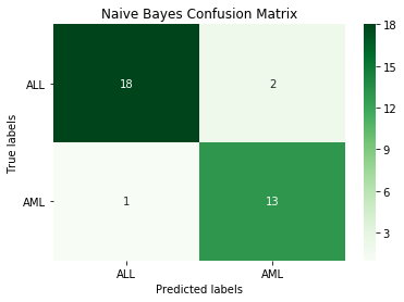
The naive bayes model is pretty good, just three incorrect classifications.

4.4 Logistic Regression

Another very standard approach is logistic regression. Here we will be using grid search cross-validation tuning to try and determine the best hyperparameters. We don't need to scale the data for logistic regression, nor are we using the PCA version of the dataset.


log_grid = {'C': [1e-03, 1e-2, 1e-1, 1, 10], 
                 'penalty': ['l1', 'l2']}

log_estimator = LogisticRegression(solver='liblinear')

log_model = GridSearchCV(estimator=log_estimator, 
                  param_grid=log_grid, 
                  cv=3,
                  scoring='accuracy')

log_model.fit(X_train, y_train.iloc[:,1])

print("Best Parameters:\n", log_model.best_params_)

# Select best log model
best_log = log_model.best_estimator_

# Make predictions using the optimised parameters
log_pred = best_log.predict(X_test)

print('Logistic Regression accuracy:', round(accuracy_score(y_test.iloc[:,1], log_pred), 3))

cm_log =  confusion_matrix(y_test.iloc[:,1], log_pred)

ax = plt.subplot()
sns.heatmap(cm_log, annot=True, ax = ax, fmt='g', cmap='Greens') 

# labels, title and ticks
ax.set_xlabel('Predicted labels')
ax.set_ylabel('True labels') 
ax.set_title('Logistic Regression Confusion Matrix') 
ax.xaxis.set_ticklabels(labels) 
ax.yaxis.set_ticklabels(labels, rotation=360);

Output:

Best Parameters:
 {'C': 1, 'penalty': 'l1'}
Logistic Regression accuracy: 1.0

LogRgene

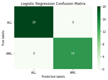
This logistic regression model manages perfect classification.

4.5 Support Vector Machine

Here we will try another traditional approach, a support vector machine (SVM) classifier. For the SVM, so we using the PCA version of the dataset. Again we use grid search cross-validation to tune the model.


# Parameter grid
svm_param_grid = {'C': [0.1, 1, 10, 100], 'gamma': [1, 0.1, 0.01, 0.001, 0.00001, 10], "kernel": ["linear", "rbf", "poly"], "decision_function_shape" : ["ovo", "ovr"]} 

# Create SVM grid search classifier
svm_grid = GridSearchCV(SVC(), svm_param_grid, cv=3)

# Train the classifier
svm_grid.fit(X_train_pca, y_train.iloc[:,1])

print("Best Parameters:\n", svm_grid.best_params_)

# Select best svc
best_svc = svm_grid.best_estimator_

# Make predictions using the optimised parameters
svm_pred = best_svc.predict(X_test_pca)

print('SVM accuracy:', round(accuracy_score(y_test.iloc[:,1], svm_pred), 3))

cm_svm =  confusion_matrix(y_test.iloc[:,1], svm_pred)

ax = plt.subplot()
sns.heatmap(cm_svm, annot=True, ax = ax, fmt='g', cmap='Greens') 

# Labels, title and ticks
ax.set_xlabel('Predicted labels')
ax.set_ylabel('True labels') 
ax.set_title('SVM Confusion Matrix') 
ax.xaxis.set_ticklabels(labels) 
ax.yaxis.set_ticklabels(labels, rotation=360);

Output:

Best Parameters:
 {'C': 0.1, 'decision_function_shape': 'ovo', 'gamma': 1, 'kernel': 'linear'}
SVM accuracy: 0.941

SVMgene

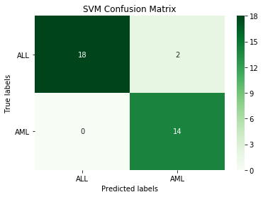
This SVM model is making just a couple of classification errors.

4.6 Neural Network

Finally we shall build a neural network using Keras (with TensorFlow as a backend). This only a "shallow" learning model with one hidden layer — adding several extra layers with so few training datapoints would just lead to overfitting.


# Create model architecture
model = Sequential()
model.add(Dense(16, activation='relu', input_shape=(7129,)))
model.add(Dense(1, activation='sigmoid'))

# Compile model
model.compile(optimizer='adam',
loss='binary_crossentropy',
metrics=['accuracy'])

# Create training/validation sets
partial_X_train = X_train_scl[:30]
X_val = X_train_scl[30:]

y_train_label = y_train.iloc[:,1]
partial_y_train = y_train_label[:30]
y_val = y_train_label[30:]

# Set up early stopping
es = EarlyStopping(monitor='val_loss', verbose=1, patience=3)

# Fit model
history = model.fit(partial_X_train,
            partial_y_train,
            epochs=50,
            batch_size=4,
            validation_data=(X_val, y_val),
            callbacks=[es])

# Make predictions
nn_pred = model.predict_classes(X_test_scl)

print('Neural Network accuracy: ', round(accuracy_score(y_test.iloc[:,1], nn_pred), 3))

cm_nn = confusion_matrix(y_test.iloc[:,1], nn_pred)

ax = plt.subplot()
sns.heatmap(cm_nn, annot=True, ax = ax, fmt='g', cmap='Greens') 

# Labels, title and ticks
ax.set_xlabel('Predicted labels')
ax.set_ylabel('True labels') 
ax.set_title('Neural Network Confusion Matrix') 
ax.xaxis.set_ticklabels(labels) 
ax.yaxis.set_ticklabels(labels, rotation=360);

Output:

Neural Network accuracy:  0.706

nngene

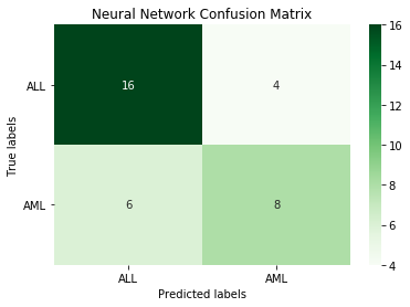
The neural network isn't as good as some of the other models.

5. Conclusion

In conclusion, the logistic regression model provided the best performance in correct molecular classification of cancer.

Complete code can be found here.

References

Golub TR, Slonim DK, Tamayo P, Huard C, Gaasenbeek M, Mesirov JP, Coller H, Loh ML, Downing JR, Caligiuri MA, Bloomfield CD, Lander ES. Molecular classification of cancer: class discovery and class prediction by gene expression monitoring. Science. 1999 Oct 15;286(5439):531-7. doi: 10.1126/science.286.5439.531. PMID: 10521349.