Graph Convolutional Neural Networks for Node Classification

gcnn

1. Introduction

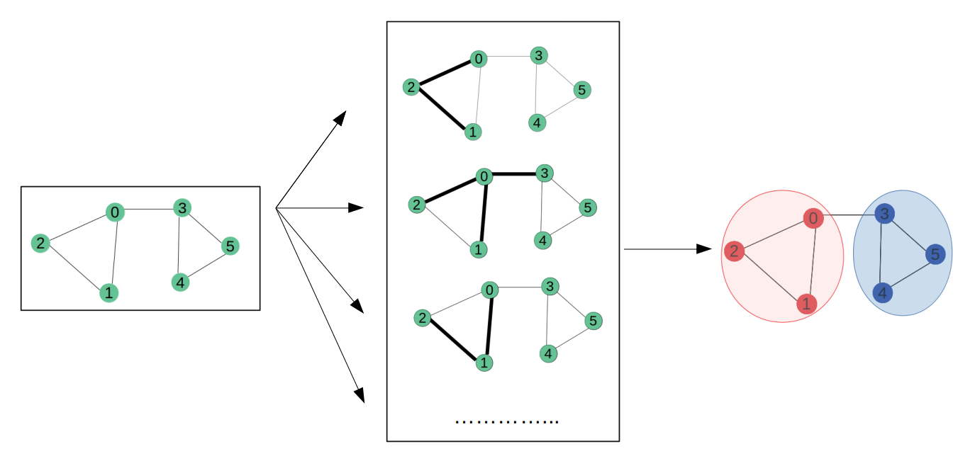
Many datasets in various machine learning (ML) applications have structural relationships between their entities, which can be represented as graphs. Such application includes social and communication networks analysis, traffic prediction, and fraud detection. Graph representation Learning aims to build and train models for graph datasets to be used for a variety of ML tasks.

This article demonstrate a simple implementation of a Graph CNN (GraphCNN) model. The model is used for a node prediction task on the Cora dataset to predict the subject of a paper given its words and citations network.

2. Import Packages


import os
import pandas as pd
import numpy as np
import networkx as nx
import matplotlib.pyplot as plt
import tensorflow as tf
from tensorflow import keras
from tensorflow.keras import layers

3. Prepare the Dataset

The Cora dataset consists of 2,708 scientific papers classified into one of seven classes. The citation network consists of 5,429 links. Each paper has a binary word vector of size 1,433, indicating the presence of a corresponding word.

3.1 Download the dataset

The dataset has two tap-separated files: cora.cites and cora.content.

1. The cora.cites includes the citation records with two columns: cited_paper_id (target) and citing_paper_id (source).

2. The cora.content includes the paper content records with 1,435 columns: paper_id, subject, and 1,433 binary features.

Let's download the dataset and below is the code for the same.


zip_file = keras.utils.get_file(
    fname="cora.tgz",
    origin="https://linqs-data.soe.ucsc.edu/public/lbc/cora.tgz",
    extract=True,
)
data_dir = os.path.join(os.path.dirname(zip_file), "cora")

3.2 Process and visualize the dataset

Then we load the citations data into a Pandas DataFrame.


citations = pd.read_csv(
    os.path.join(data_dir, "cora.cites"),
    sep="\t",
    header=None,
    names=["target", "source"],
)
print("Citations shape:", citations.shape)


Citations shape: (5429, 2)

Here we can see a sample of the "citations" DataFrame. The target column includes the paper ids cited by the paper ids in the "source" column.


citations.sample(frac=1).head())

Table below shows some sample data.

	target	source
2581	28227	6169
1500	7297	7276
1194	6184	1105718
4221	139738	1108834
3707	79809	1153275

Let's load the papers data into a Pandas DataFrame.


column_names = ["paper_id"] + [f"term_{idx}" for idx in range(1433)] + ["subject"]
papers = pd.read_csv(
    os.path.join(data_dir, "cora.content"), sep="\t", header=None, names=column_names,
)
print("Papers shape:", papers.shape)


Papers shape: (2708, 1435)

Below we print a dataFrame that includes the paper_id and the subject columns, as well as 1,433 binary column representing whether a term exists in the paper or not.


print(papers.sample(5).T)

Figure below shows the dataframe for paper_id and subject_id.

paperid

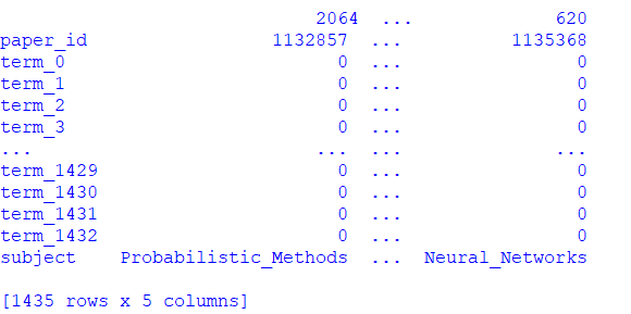
Figure 1. Dataframe for paper_id and subject_id.

Let's display the count of the papers in each subject.


print(papers.subject.value_counts())

Figure below shows the count of the papers in each subject .

papers

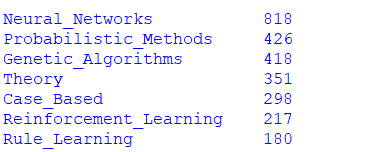
Figure 2. Count of the papers in each subject.

Now we will convert the paper ids and the subjects into zero-based indices.


class_values = sorted(papers["subject"].unique())
class_idx = {name: id for id, name in enumerate(class_values)}
paper_idx = {name: idx for idx, name in enumerate(sorted(papers["paper_id"].unique()))}

papers["paper_id"] = papers["paper_id"].apply(lambda name: paper_idx[name])
citations["source"] = citations["source"].apply(lambda name: paper_idx[name])
citations["target"] = citations["target"].apply(lambda name: paper_idx[name])
papers["subject"] = papers["subject"].apply(lambda value: class_idx[value])

Now let's visualize the citation graph. Each node in the graph represents a paper, and the color of the node corresponds to its subject. Note that we only show a sample of the papers in the dataset.


plt.figure(figsize=(10, 10))
colors = papers["subject"].tolist()
cora_graph = nx.from_pandas_edgelist(citations.sample(n=1500))
subjects = list(papers[papers["paper_id"].isin(list(cora_graph.nodes))]["subject"])
nx.draw_spring(cora_graph, node_size=15, node_color=subjects)

Figure below shows the citation graph.

nodes

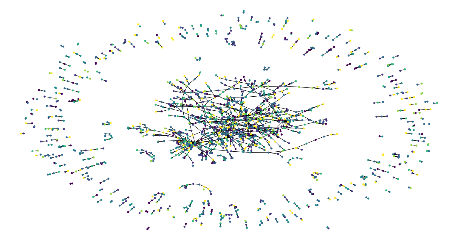
Figure 3. Citation graph.

4. Data Pre-Processing


train_data, test_data = [], []
for _, group_data in papers.groupby("subject"):
    # Select around 50% of the dataset for training.
    random_selection = np.random.rand(len(group_data.index)) <= 0.5
    train_data.append(group_data[random_selection])
    test_data.append(group_data[~random_selection])

train_data = pd.concat(train_data).sample(frac=1)
test_data = pd.concat(test_data).sample(frac=1)

print("Train data shape:", train_data.shape)
print("Test data shape:", test_data.shape)


Train data shape: (1360, 1435)
Test data shape: (1348, 1435

This function displays the loss and accuracy curves of the model during training.



def display_learning_curves(history):
    fig, (ax1, ax2) = plt.subplots(1, 2, figsize=(15, 5))

    ax1.plot(history.history["loss"])
    ax1.plot(history.history["val_loss"])
    ax1.legend(["train", "test"], loc="upper right")
    ax1.set_xlabel("Epochs")
    ax1.set_ylabel("Loss")

    ax2.plot(history.history["acc"])
    ax2.plot(history.history["val_acc"])
    ax2.legend(["train", "test"], loc="upper right")
    ax2.set_xlabel("Epochs")
    ax2.set_ylabel("Accuracy")
    plt.show()

5. Building a Graph Neural Network Model

5.1 Prepare the data for the graph model

Preparing and loading the graphs data into the model for training is the most challenging part in GNN models, which is addressed in different ways by the specialised libraries. In this example, we show a simple approach for preparing and using graph data that is suitable if your dataset consists of a single graph that fits entirely in memory.

The graph data is represented by the graph_info tuple, which consists of the following three elements:

1. node_features: This is a [num_nodes, num_features] NumPy array that includes the node features. In this dataset, the nodes are the papers, and the node_features are the word-presence binary vectors of each paper.

2. edges: This is [num_edges, num_edges] NumPy array representing a sparse adjacency matrix of the links between the nodes. In this example, the links are the citations between the papers.

3. edge_weights: This is a [num_edges] NumPy array that includes the edge weights, which quantify the relationships between nodes in the graph. In this example, there are no weights for the paper citations.


# Create an edges array (sparse adjacency matrix) of shape [2, num_edges].
edges = citations[["source", "target"]].to_numpy().T
# Create an edge weights array of ones.
edge_weights = tf.ones(shape=edges.shape[1])
# Create a node features array of shape [num_nodes, num_features].
node_features = tf.cast(
    papers.sort_values("paper_id")[feature_names].to_numpy(), dtype=tf.dtypes.float32
)
# Create graph info tuple with node_features, edges, and edge_weights.
graph_info = (node_features, edges, edge_weights)

print("Edges shape:", edges.shape)
print("Nodes shape:", node_features.shape)

OUTPUT:
Edges shape: (2, 5429)
Nodes shape: (2708, 1433)

5.2 Implement a graph convolution layer

We implement a graph convolution module as a Keras Layer. Our GraphConvLayer performs the following steps:

1. Prepare: The input node representations are processed using a FFN to produce a message. You can simplify the processing by only applying linear transformation to the representations.

2. Aggregate: The messages of the neighbours of each node are aggregated with respect to the edge_weights using a permutation invariant pooling operation, such as sum, mean, and max, to prepare a single aggregated message for each node. See, for example, tf.math.unsorted_segment_sum APIs used to aggregate neighbour messages.

3. Update: The node_repesentations and aggregated_messages—both of shape [num_nodes, representation_dim]— are combined and processed to produce the new state of the node representations (node embeddings). If combination_type is gru, the node_repesentations and aggregated_messages are stacked to create a sequence, then processed by a GRU layer. Otherwise, the node_repesentations and aggregated_messages are added or concatenated, then processed using a FFN.

The technique implemented use ideas from Graph Convolutional Networks, GraphSage, Graph Isomorphism Network, Simple Graph Networks, and Gated Graph Sequence Neural Networks.


class GraphConvLayer(layers.Layer):
    def __init__(
        self,
        hidden_units,
        dropout_rate=0.2,
        aggregation_type="mean",
        combination_type="concat",
        normalize=False,
        *args,
        **kwargs,
    ):
        super(GraphConvLayer, self).__init__(*args, **kwargs)

        self.aggregation_type = aggregation_type
        self.combination_type = combination_type
        self.normalize = normalize

        self.ffn_prepare = create_ffn(hidden_units, dropout_rate)
        if self.combination_type == "gated":
            self.update_fn = layers.GRU(
                units=hidden_units,
                activation="tanh",
                recurrent_activation="sigmoid",
                dropout=dropout_rate,
                return_state=True,
                recurrent_dropout=dropout_rate,
            )
        else:
            self.update_fn = create_ffn(hidden_units, dropout_rate)

    def prepare(self, node_repesentations, weights=None):
        # node_repesentations shape is [num_edges, embedding_dim].
        messages = self.ffn_prepare(node_repesentations)
        if weights is not None:
            messages = messages * tf.expand_dims(weights, -1)
        return messages

    def aggregate(self, node_indices, neighbour_messages):
        # node_indices shape is [num_edges].
        # neighbour_messages shape: [num_edges, representation_dim].
        num_nodes = tf.math.reduce_max(node_indices) + 1
        if self.aggregation_type == "sum":
            aggregated_message = tf.math.unsorted_segment_sum(
                neighbour_messages, node_indices, num_segments=num_nodes
            )
        elif self.aggregation_type == "mean":
            aggregated_message = tf.math.unsorted_segment_mean(
                neighbour_messages, node_indices, num_segments=num_nodes
            )
        elif self.aggregation_type == "max":
            aggregated_message = tf.math.unsorted_segment_max(
                neighbour_messages, node_indices, num_segments=num_nodes
            )
        else:
            raise ValueError(f"Invalid aggregation type: {self.aggregation_type}.")

        return aggregated_message

    def update(self, node_repesentations, aggregated_messages):
        # node_repesentations shape is [num_nodes, representation_dim].
        # aggregated_messages shape is [num_nodes, representation_dim].
        if self.combination_type == "gru":
            # Create a sequence of two elements for the GRU layer.
            h = tf.stack([node_repesentations, aggregated_messages], axis=1)
        elif self.combination_type == "concat":
            # Concatenate the node_repesentations and aggregated_messages.
            h = tf.concat([node_repesentations, aggregated_messages], axis=1)
        elif self.combination_type == "add":
            # Add node_repesentations and aggregated_messages.
            h = node_repesentations + aggregated_messages
        else:
            raise ValueError(f"Invalid combination type: {self.combination_type}.")

        # Apply the processing function.
        node_embeddings = self.update_fn(h)
        if self.combination_type == "gru":
            node_embeddings = tf.unstack(node_embeddings, axis=1)[-1]

        if self.normalize:
            node_embeddings = tf.nn.l2_normalize(node_embeddings, axis=-1)
        return node_embeddings

    def call(self, inputs):
        """Process the inputs to produce the node_embeddings.

        inputs: a tuple of three elements: node_repesentations, edges, edge_weights.
        Returns: node_embeddings of shape [num_nodes, representation_dim].
        """

        node_repesentations, edges, edge_weights = inputs
        # Get node_indices (source) and neighbour_indices (target) from edges.
        node_indices, neighbour_indices = edges[0], edges[1]
        # neighbour_repesentations shape is [num_edges, representation_dim].
        neighbour_repesentations = tf.gather(node_repesentations, neighbour_indices)

        # Prepare the messages of the neighbours.
        neighbour_messages = self.prepare(neighbour_repesentations, edge_weights)
        # Aggregate the neighbour messages.
        aggregated_messages = self.aggregate(node_indices, neighbour_messages)
        # Update the node embedding with the neighbour messages.
        return self.update(node_repesentations, aggregated_messages)

5.3 Implement a graph neural network node classifier

The GNN classification model follows the Design Space for Graph Neural Networks approach, as follows:

1. Apply preprocessing to the node features to generate initial node representations.

2. Apply one or more graph convolutional layer, with skip connections, to the node representation to produce node embeddings.

3. Apply post-processing to the node embeddings to generat the final node embeddings.

4. Feed the node embeddings in a Softmax layer to predict the node class.

Each graph convolutional layer added captures information from a further level of neighbours. However, adding many graph convolutional layer can cause oversmoothing, where the model produces similar embeddings for all the nodes.

Note that the graph_info passed to the constructor of the Keras model, and used as a property of the Keras model object, rather than input data for training or prediction. The model will accept a batch of node_indices, which are used to lookup the node features and neighbours from the graph_info.


class GNNNodeClassifier(tf.keras.Model):
    def __init__(
        self,
        graph_info,
        num_classes,
        hidden_units,
        aggregation_type="sum",
        combination_type="concat",
        dropout_rate=0.2,
        normalize=True,
        *args,
        **kwargs,
    ):
        super(GNNNodeClassifier, self).__init__(*args, **kwargs)

        # Unpack graph_info to three elements: node_features, edges, and edge_weight.
        node_features, edges, edge_weights = graph_info
        self.node_features = node_features
        self.edges = edges
        self.edge_weights = edge_weights
        # Set edge_weights to ones if not provided.
        if self.edge_weights is None:
            self.edge_weights = tf.ones(shape=edges.shape[1])
        # Scale edge_weights to sum to 1.
        self.edge_weights = self.edge_weights / tf.math.reduce_sum(self.edge_weights)

        # Create a process layer.
        self.preprocess = create_ffn(hidden_units, dropout_rate, name="preprocess")
        # Create the first GraphConv layer.
        self.conv1 = GraphConvLayer(
            hidden_units,
            dropout_rate,
            aggregation_type,
            combination_type,
            normalize,
            name="graph_conv1",
        )
        # Create the second GraphConv layer.
        self.conv2 = GraphConvLayer(
            hidden_units,
            dropout_rate,
            aggregation_type,
            combination_type,
            normalize,
            name="graph_conv2",
        )
        # Create a postprocess layer.
        self.postprocess = create_ffn(hidden_units, dropout_rate, name="postprocess")
        # Create a compute logits layer.
        self.compute_logits = layers.Dense(units=num_classes, name="logits")

    def call(self, input_node_indices):
        # Preprocess the node_features to produce node representations.
        x = self.preprocess(self.node_features)
        # Apply the first graph conv layer.
        x1 = self.conv1((x, self.edges, self.edge_weights))
        # Skip connection.
        x = x1 + x
        # Apply the second graph conv layer.
        x2 = self.conv2((x, self.edges, self.edge_weights))
        # Skip connection.
        x = x2 + x
        # Postprocess node embedding.
        x = self.postprocess(x)
        # Fetch node embeddings for the input node_indices.
        node_embeddings = tf.squeeze(tf.gather(x, input_node_indices))
        # Compute logits
        return self.compute_logits(node_embeddings)

Let's test instantiating and calling the GNN model. Notice that if you provide N node indices, the output will be a tensor of shape [N, num_classes], regardless of the size of the graph.


gnn_model = GNNNodeClassifier(
    graph_info=graph_info,
    num_classes=num_classes,
    hidden_units=hidden_units,
    dropout_rate=dropout_rate,
    name="gnn_model",
)

print("GNN output shape:", gnn_model([1, 10, 100]))

gnn_model.summary()

Figure below shows the build model summary.

model_summary

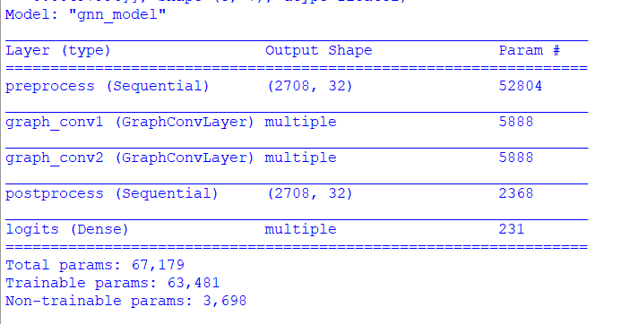
Figure 4. Model summary.

5.4 Training the GNN model

Note that we use the standard supervised cross-entropy loss to train the model. However, we can add another self-supervised loss term for the generated node embeddings that makes sure that neighbouring nodes in graph have similar representations, while faraway nodes have dissimilar representations.


x_train = train_data.paper_id.to_numpy()
history = run_experiment(gnn_model, x_train, y_train)

Plotting the learning curves.


display_learning_curves(history)

Figure below shows the learning curves for the Graph CNN model.

learning_curve

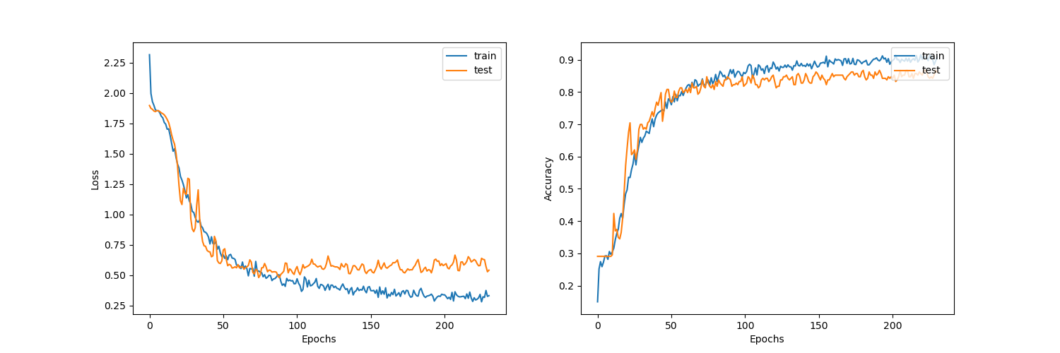
Figure 5. GraphCNN learning curves.

Now we evaluate the GNN model on the test data split. The results may vary depending on the training sample, however the GNN model always outperforms the baseline model in terms of the test accuracy.


x_test = test_data.paper_id.to_numpy()
_, test_accuracy = gnn_model.evaluate(x=x_test, y=y_test, verbose=0)
print(f"Test accuracy: {round(test_accuracy * 100, 2)}%")
Test accuracy: 80.19%

5.5 Examine the GNN model predictions

Let's add the new instances as nodes to the node_features, and generate links (citations) to existing nodes.


 First we add the N new_instances as nodes to the graph
# by appending the new_instance to node_features.
num_nodes = node_features.shape[0]
new_node_features = np.concatenate([node_features, new_instances])
# Second we add the M edges (citations) from each new node to a set
# of existing nodes in a particular subject
new_node_indices = [i + num_nodes for i in range(num_classes)]
new_citations = []
for subject_idx, group in papers.groupby("subject"):
    subject_papers = list(group.paper_id)
    # Select random x papers specific subject.
    selected_paper_indices1 = np.random.choice(subject_papers, 5)
    # Select random y papers from any subject (where y < x).
    selected_paper_indices2 = np.random.choice(list(papers.paper_id), 2)
    # Merge the selected paper indices.
    selected_paper_indices = np.concatenate(
        [selected_paper_indices1, selected_paper_indices2], axis=0
    )
    # Create edges between a citing paper idx and the selected cited papers.
    citing_paper_indx = new_node_indices[subject_idx]
    for cited_paper_idx in selected_paper_indices:
        new_citations.append([citing_paper_indx, cited_paper_idx])

new_citations = np.array(new_citations).T
new_edges = np.concatenate([edges, new_citations], axis=1)

# Updating the node_features and the edges in the GNN model.

print("Original node_features shape:", gnn_model.node_features.shape)
print("Original edges shape:", gnn_model.edges.shape)
gnn_model.node_features = new_node_features
gnn_model.edges = new_edges
gnn_model.edge_weights = tf.ones(shape=new_edges.shape[1])
print("New node_features shape:", gnn_model.node_features.shape)
print("New edges shape:", gnn_model.edges.shape)

logits = gnn_model.predict(tf.convert_to_tensor(new_node_indices))
probabilities = keras.activations.softmax(tf.convert_to_tensor(logits)).numpy()
display_class_probabilities(probabilities)


OUTPUT:
Original node_features shape: (2708, 1433)
Original edges shape: (2, 5429)
New node_features shape: (2715, 1433)
New edges shape: (2, 5478)
Instance 1:
- Case_Based: 4.35%
- Genetic_Algorithms: 4.19%
- Neural_Networks: 1.49%
- Probabilistic_Methods: 1.68%
- Reinforcement_Learning: 21.34%
- Rule_Learning: 52.82%
- Theory: 14.14%
Instance 2:
- Case_Based: 0.01%
- Genetic_Algorithms: 99.88%
- Neural_Networks: 0.03%
- Probabilistic_Methods: 0.0%
- Reinforcement_Learning: 0.07%
- Rule_Learning: 0.0%
- Theory: 0.01%
Instance 3:
- Case_Based: 0.1%
- Genetic_Algorithms: 59.18%
- Neural_Networks: 39.17%
- Probabilistic_Methods: 0.38%
- Reinforcement_Learning: 0.55%
- Rule_Learning: 0.08%
- Theory: 0.54%
Instance 4:
- Case_Based: 0.14%
- Genetic_Algorithms: 10.44%
- Neural_Networks: 84.1%
- Probabilistic_Methods: 3.61%
- Reinforcement_Learning: 0.71%
- Rule_Learning: 0.16%
- Theory: 0.85%
Instance 5:
- Case_Based: 0.27%
- Genetic_Algorithms: 0.15%
- Neural_Networks: 0.48%
- Probabilistic_Methods: 0.23%
- Reinforcement_Learning: 0.79%
- Rule_Learning: 0.45%
- Theory: 97.63%
Instance 6:
- Case_Based: 3.12%
- Genetic_Algorithms: 1.35%
- Neural_Networks: 19.72%
- Probabilistic_Methods: 0.48%
- Reinforcement_Learning: 39.56%
- Rule_Learning: 28.0%
- Theory: 7.77%
Instance 7:
- Case_Based: 1.6%
- Genetic_Algorithms: 34.76%
- Neural_Networks: 4.45%
- Probabilistic_Methods: 9.59%
- Reinforcement_Learning: 2.97%
- Rule_Learning: 4.05%
- Theory: 42.6%

Here, we see that the probabilities of the expected subjects (to which several citations are added) are higher compared to the baseline model.

6. Conclusion

In this article, we build and tested our Graph Convolutional Neural Network (GraphCNN) model for the node classification task. Our proposed model achieved an accuracy of 80% in correct classification of the nodes.

References

Ma, T., Wang, H., Zhang, L., Tian, Y., & Al-Nabhan, N. (2021). Graph classification based on structural features of significant nodes and spatial convolutional neural networks. Neurocomputing, 423, 639-650.
Cangea, C., Veličković, P., Jovanović, N., Kipf, T., & Liò, P. (2018). Towards sparse hierarchical graph classifiers. arXiv preprint arXiv:1811.01287.