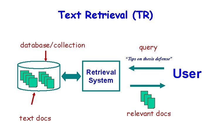
Natural Language Processing Based Text Retrieval System

TR0

1. Introduction

The term Text retrieval can be stated as the matching of some user generated query against a set of text records. These records could be any type such as: unstructured text, documentations, textual-reports, newspaper articles, paragraphs in a manual, etc. User queries can range from multi-sentence full descriptions of an information need to just a few words. Text retrieval is a subset of Information retrieval systems. Search engines like Google, Bing, etc. are example of such systems.

This article will introduce techniques for organizing text data. It will show how to analyze a large corpus of text, extracting feature vectors for individual documents, in order to be able to retrieve documents with similar content.

2. Prerequisite

Python and Scikit-learn, Scipy packages are required to run through this article, as well as a corpus of text documents. This code can be adapted to work with other set of documents we collect.

3. Datset

We will use the well-known Reuters-21578 dataset. It includes 12,902 documents for 90 classes, with a fixed splitting between test and training data (3,299, 9,603). To obtain from it the Reuters 10 categories Apte' split it is enough to select the 10 top-sized categories, i.e. Earn, Acquisition, Money-fx, Grain, Crude, Trade, Interest, Ship, Wheat, and Corn. The dataset can be downloaded from here.

Once we have downloaded and unzipped the dataset, we can take a look inside the folder. It is split into two folders, "training" and "test". Each of those contains 91 subfolders, corresponding to pre-labeled categories, which will be useful for us later when we want to try classifying the category of an unknown message. In this article, we are not worried about training a classifier, so we'll end up using both sets together.

4. Methodology

In this section we will perform data exploration, data pre-processing, text-vectorization, and text-analysis steps.

4.1 Data Exploration

Let's open up a single message and look at the contents. This is the very first message in the training folder, inside of the "acq" folder, which is a category apparently containing news of corporate acquisitions.


import os
dataset= '../Text_data/Reuters21578-Apte-90Cat'

post_path = os.path.join(dataset, "training", "acq", "0000005")
with open (post_path, "r") as p:
    raw_text = p.read()
    print(raw_text)

Figure below shows a single sample message.

TR1

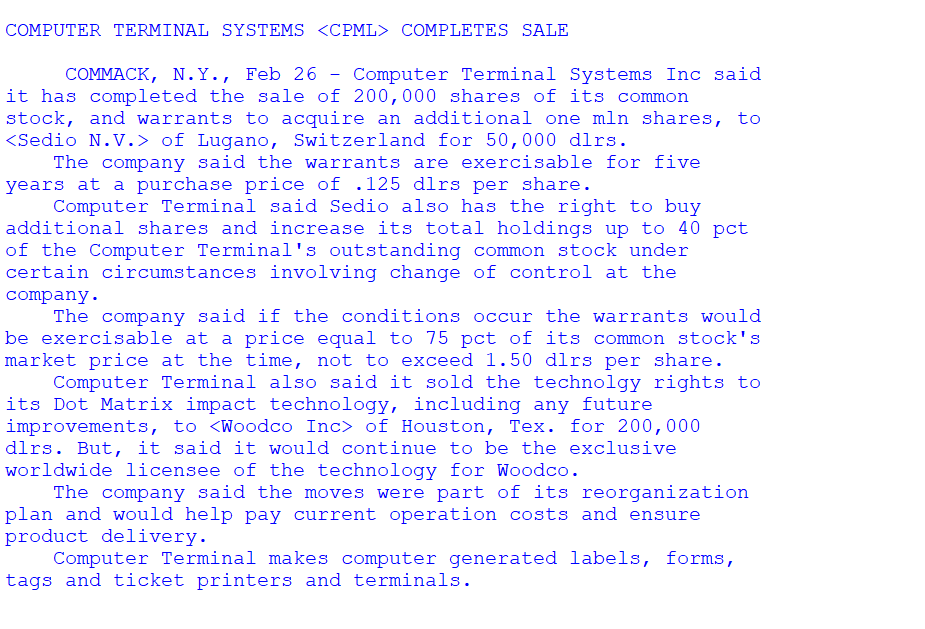
Figure 1. sample message

4.2 Data Pre-Processing

Our collection contains over 15,000 articles with a lot of information. It would take way too long to get through all the information.


# this gives us all the groups (from training subfolder, but same for test)
groups = [g for g in os.listdir(os.path.join(data_dir, "training")) if os.path.isdir(os.path.join(data_dir, "training", g))]
print groups

Figure below shows the different groups present in our dataset.

TR2

Figure 2. Different groups present in our dataset

Let's load all of our documents (news articles) into a single list called docs. We'll iterate through each group, grab all of the posts in each group (from both training and test directories), and add the text of the post into the docs list. We will make sure to exclude duplicate posts by cheking if we've seen the post index before.


import re

docs = []
post_idx = []
for g, group in enumerate(groups):
    if g%10==0:
        print ("reading group %d / %d"%(g+1, len(groups)))
    posts_training = [os.path.join(data_dir, "training", group, p) for p in os.listdir(os.path.join(data_dir, "training", group)) if os.path.isfile(os.path.join(data_dir, "training", group, p))]
    posts_test = [os.path.join(data_dir, "test", group, p) for p in os.listdir(os.path.join(data_dir, "test", group)) if os.path.isfile(os.path.join(data_dir, "test", group, p))]
    posts = posts_training + posts_test
    for post in posts:
        idx = post.split("/")[-1]
        if idx not in post_idx:
            post_idx.append(idx)
            with open(post, "r") as p:
                raw_text = p.read()
                raw_text = re.sub(r'[^\x00-\x7f]',r'', raw_text) 
                docs.append(raw_text)

print("\nwe have %d documents in %d groups"%(len(docs), len(groups)))
print("\nhere is document 100:\n%s"%docs[100])

Figure below shows the output of above code and content of document number 100.

TR3

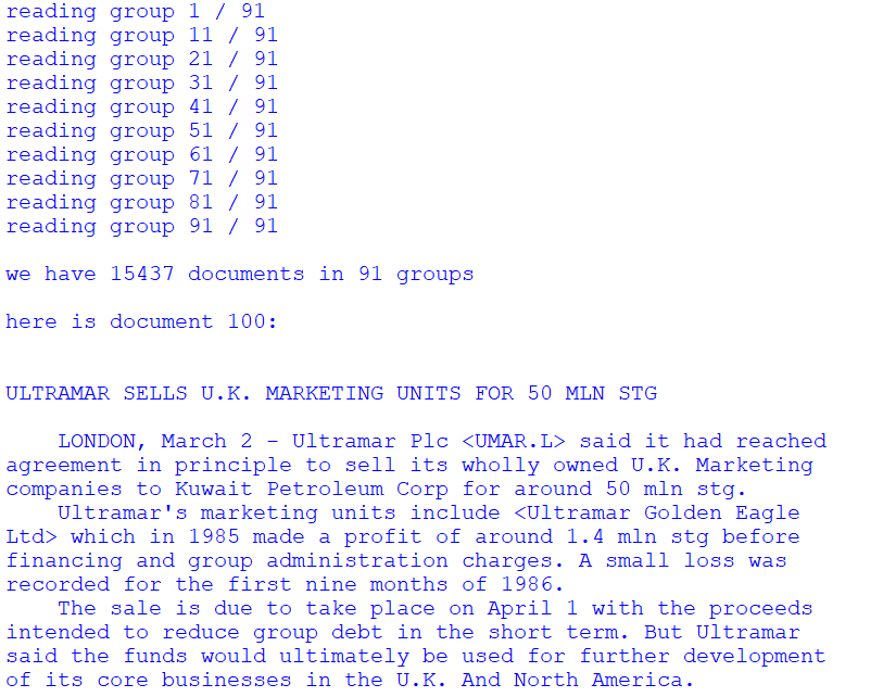
Figure 3. Content of document number 100

4.3 Text Vectorization

We will now use sklearn's TfidfVectorizer to compute the tf-idf matrix of our collection of documents. The tf-idf matrix is an n*m matrix with the n rows corresponding to our n documents and the m columns corresponding to our terms.

The values corresponds to the "importance" of each term to each document, where importance is *. In this case, terms are just all the unique words in the corpus, minus english _stopwords_, which are the most common words in the english language, e.g. "it", "they", "and", "a", etc. In some cases, terms can be n-grams (n-length sequences of words) or more complex, but usually just words.

To compute the tf-idf matrix, run:


from sklearn.feature_extraction.text import TfidfVectorizer
vectorizer = TfidfVectorizer(stop_words='english')
tfidf = vectorizer.fit_transform(docs)

TR4

Figure 4. TfIdf vectorizer

We see that the variable tfidf is a sparse matrix with a row for each document, and a column for each unique term in the corpus.

Thus, we can interpret each row of this matrix as a feature vector which describes a document. Two documents which have identical rows have the same collection of words in them, although not necessarily in the same order; word order is not preserved in the tf-idf matrix. Regardless, it seems reasonable to expect that if two documents have similar or close tf-idf vectors, they probably have similar content.


doc_idx = 5
doc_tfidf = tfidf.getrow(doc_idx)
all_terms = vectorizer.get_feature_names()
terms = [all_terms[i] for i in doc_tfidf.indices]
values = doc_tfidf.data

print(docs[doc_idx])
print("document's term-frequency pairs:")
print(", ".join("\"%s\"=%0.2f"%(t,v) for t,v in zip(terms,values)))

TR5

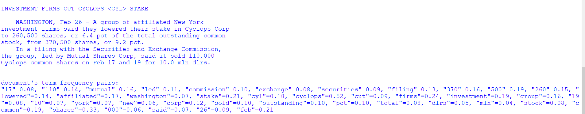
Figure 5. TfIdf vector values for document id:5

4.4 Text Analysis

In practice however, the term-document matrix alone has several disadvantages. For one, it is very high-dimensional and sparse (mostly zeroes), thus it is computationally costly.

Additionally, it ignores similarity among groups of terms. For example, the words "seat" and "chair" are related, but in a raw term-document matrix they are separate columns. So two sentences with one of each word will not be computed as similarly.

One solution is to use latent semantic analysis (LSA, or sometimes called latent semantic indexing). LSA is a dimensionality reduction technique closely related to principal component analysis, which is commonly used to reduce a high-dimensional set of terms into a lower-dimensional set of "concepts" or components which are linear combinations of the terms.

To do so, we use sklearn's "TruncatedSVD" function which gives us the LSA by computing a singular value decomposition (SVD) of the tf-idf matrix.


from sklearn.decomposition import TruncatedSVD

lsa = TruncatedSVD(n_components=100)
tfidf_lsa = lsa.fit_transform(tfidf)

How to interpret this? "lsa" holds our latent semantic analysis, expressing our 100 concepts. It has a vector for each concept, which holds the weight of each term to that concept. "tfidf_lsa" is our transformed document matrix where each document is a weighted sum of the concepts.

In a simpler analysis with, for example, two topics (sports and tacos), one concept might assign high weights for sports-related terms (ball, score, tournament) and the other one might have high weights for taco-related concepts (cheese, tomato, lettuce). In a more complex one like this one, the concepts may not be as interpretable. Nevertheless, we can investigate the weights for each concept, and look at the top-weighted ones. For example, below here are the top terms in concept 1.


components = lsa.components_[1]
all_terms = vectorizer.get_feature_names()

idx_top_terms = sorted(range(len(components)), key=lambda k: components[k])

print("10 highest-weighted terms in concept 1:")
for t in idx_top_terms[:10]:
    print(" - %s : %0.02f"%(all_terms[t], t))

TR6

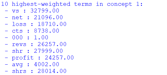
Figure 6. Ten highest-weighted terms in concept 1

The top terms in concept 1 appear related to accounting balance sheets; terms like "net", "loss", "profit".

Now, back to our documents. Recall that tfidf_lsa is a transformation of our original tf-idf matrix from the term-space into a concept-space. The concept space is much more valuable, and we can use it to query most similar documents. We expect that two documents which about similar things should have similar vectors in tfidf_lsa. We can use a simple distance metric to measure the similarity, euclidean distance or cosine similarity being the two most common.

Here, we'll select a single query document (index 300), calculate the distance of every other document to our query document, and take the one with the smallest distance to the query.


from scipy.spatial import distance

query_idx = 400

# take the concept representation of our query document
query_features = tfidf_lsa[query_idx]

# calculate the distance between query and every other document
distances = [ distance.euclidean(query_features, feat) for feat in tfidf_lsa ]
    
# sort indices by distances, excluding the first one which is distance from query to itself (0)
idx_closest = sorted(range(len(distances)), key=lambda k: distances[k])[1:]

# print our results
query_doc = docs[query_idx]
return_doc = docs[idx_closest[0]]
print("QUERY DOCUMENT:\n %s \nMOST SIMILAR DOCUMENT TO QUERY:\n %s" %(query_doc, return_doc))

Figure below shows the Query document.

TR7

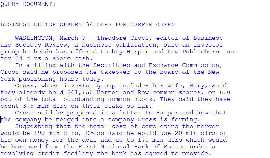
Figure 7. Query document

Figure below shows the most similar document to the query.

TR8

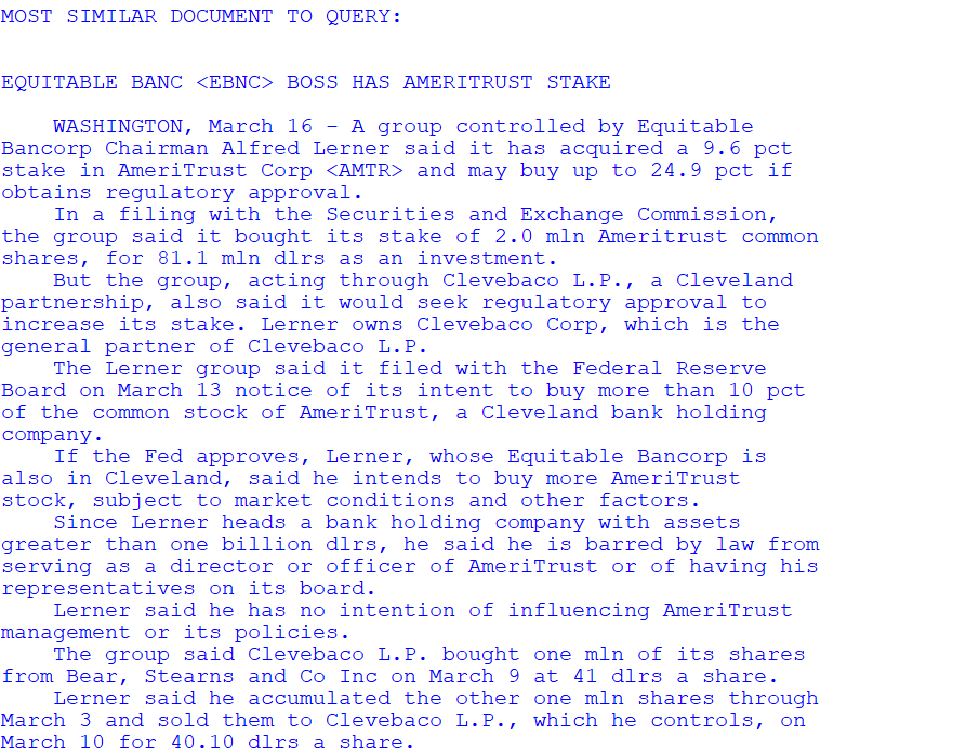
Figure 8. Most similar document to query

5. Generating Wordcloud!!!

Here for generating wordcloud we will use "Wordcloud" package available in python. We will extract the textual data for the first 100 documents and remove the stopwards present in the same using the "STOPWORDS" package. Furthermore, we will use "matplotlib" package for plotting the generated wordcloud. Below is the code for the same.


#Generating Wordcloud for the first 100 docs.
text_data=[]
for i in range(100):
	text=docs[i]
	text_data.append(text)

from wordcloud import WordCloud, STOPWORDS
import matplotlib.pyplot as plt

text = ' '.join(text_data)
stopwords = set(STOPWORDS) 
wordcloud = WordCloud( stopwords=stopwords, background_color="white",width=1600,height=1000).generate(text)

##Plotting
plt.figure(figsize=(20,10))
plt.axis("off")

# "bilinear" interpolation is used to make the displayed image appear more smoothly without overlapping of words  
# can change to some other interpolation technique to see changes like "hamming"
plt.imshow(wordcloud, interpolation="bilinear") 
plt.show()

Figure below shows the wordcloud generated from the first 100 documents.

TR9

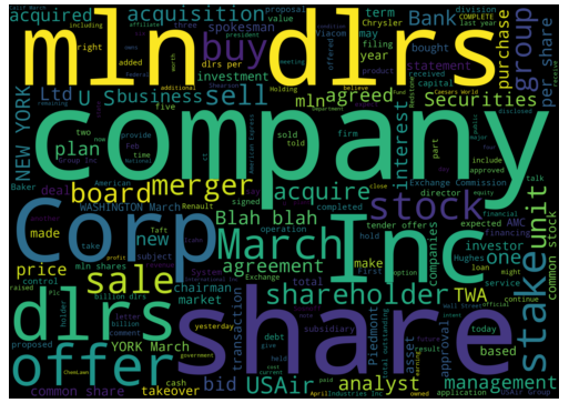
Figure 9. Wordcloud

6. Conclusion

Interesting find! Our query document appears to be about buying a stake. Our return document is a related article about the same topic. Try looking at the next few closest results. A quick inspection reveals that most of them are about the same story.

Thus we see the value of this procedure. It gives us a way to quickly identify articles which are related to each other. This can greatly aide journalists who have to sift through a lot of content which is not always indexed or organized usefully.

Complete code can be found here.

References

Robertson, S. E., & Spärck Jones, K. (1994). Simple, proven approaches to text retrieval (No. UCAM-CL-TR-356). University of Cambridge, Computer Laboratory.