Though many phenomena in the world can be well-modeled using basic linear regression or classification, there are also many interesting phenomena that are nonlinear in nature. In order to deal with nonlinear phenomena, there have been a diversity of nonlinear models developed.
For example parametric models assume that data follow some parametric class of nonlinear function (e.g. polynomial, power, or exponential), then fine-tune the shape of the parametric function to fit observed data. However this approach is only helpful if data are fit nicely by the available catalog of parametric functions.
Another approach, kernel-based methods, transforms data non-linearly into an abstract space that measures distances between observations, then predicts new values or classes based on these distances. However, kernel methods generally involve constructing a kernel matrix that depends on the number of training observations and can thus be prohibitive for large data sets.
Another class of models, the ones that are the focus of this post, are artificial neural networks (ANNs). ANNs are nonlinear models motivated by the physiological architecture of the nervous system. They involve a cascade of simple nonlinear computations that, when aggregated, can implement robust and complex nonlinear functions. In fact, depending on how they are constructed, ANNs can approximate any nonlinear function, making them a quite powerful class of models1.
In recent years ANNs that use multiple stages of nonlinear computation (aka “deep learning”) have been able obtain outstanding performance on an array of complex tasks ranging from visual object recognition to natural language processing. I find ANNs super interesting due to their computational power and their intersection with computational neuroscience. However, I’ve found that most of the available tutorials on ANNs are either dense with formal details and contain little information about implementation or any examples, while others skip a lot of the mathematical detail and provide implementations that seem to come from thin air. This post aims at giving a more complete overview of ANNs, including (varying degrees of) the math behind ANNs, how ANNs are implemented in code, and finally some toy examples that point out the strengths and weaknesses of ANNs.
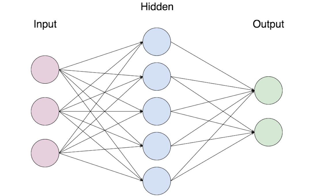
Single-layer Neural Networks
The simplest ANN (Figure 1) takes a set of observed inputs \(\mathbf{a}=(a_1, a_2, ..., a_N)\), multiplies each of them by their own associated weight \(\mathbf{w} = (w_1, w_2, ...w_N)\) , and sums the weighted values to form a pre-activation \(z\). Oftentimes there is also a bias \(b\) that is tied to an input that is always +1 included in the preactivation calculation. The network then transforms the pre-activation using a nonlinear activation function \(g(z)\) to output a final activation \(a_{\text{out}}\).
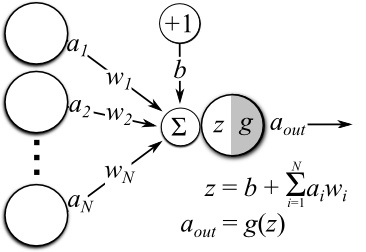
Figure 1: Diagram of a single-layered artificial neural network.
There are many options available for the form of the activation function \(g(z)\), and the choice generally depends on the task we would like the network to perform. For instance, if the activation function is the identity function:
\[g_{\text{linear}}(z) = z\]which outputs continuous values \(a_{linear}\in (-\infty, \infty)\), then the network implements a linear model akin to used in standard linear regression. Another choice for the activation function is the logistic sigmoid:
\[g_{\text{logistic}}(z) = \frac{1}{1+e^{-z}}\]which outputs values \(a_{logistic} \in (0,1)\). When the network outputs use the logistic sigmoid activation function, the network implements linear binary classification. Binary classification can also be implemented using the hyperbolic tangent function, \(\text{tanh}(z)\), which outputs values \(a_{\text{tanh}}\in (-1, 1)\) (note that the classes must also be coded as either -1 or 1 when using \(\text{tanh}\). Single-layered neural networks used for classification are often referred to as “perceptrons,” a name given to them when they were first developed in the late 1950s.
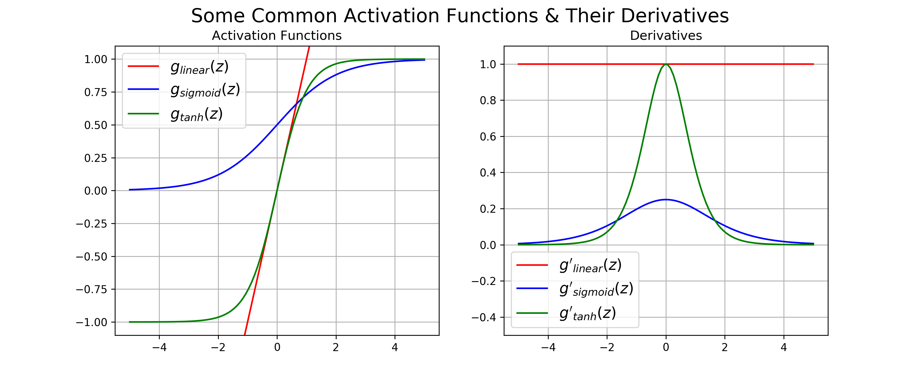
Figure 2: Common activation functions functions used in artificial neural, along with their derivatives
Python Code
import numpy as np
from matplotlib import pyplot as plt
from collections import OrderedDict

# Define a few common activation functions
g_linear = lambda z: z
g_sigmoid = lambda z: 1./(1. + np.exp(-z))
g_tanh = lambda z: np.tanh(z)

# ...and their analytic derivatives
g_prime_linear = lambda z: np.ones(len(z))
g_prime_sigmoid = lambda z: 1./(1 + np.exp(-z)) * (1 - 1./(1 + np.exp(-z)))
g_prime_tanh = lambda z: 1 - np.tanh(z) ** 2

# Visualize each g_*(z)
activation_functions = OrderedDict(
    [
        ("linear", (g_linear, g_prime_linear, 'red')),
        ("sigmoid", (g_sigmoid, g_prime_sigmoid, 'blue')),
        ("tanh", (g_tanh, g_prime_tanh, 'green')),
    ]
)

fig, axs = plt.subplots(1, 2, figsize=(12, 5))
xs = np.linspace(-5, 5, 100)
for name, params in activation_functions.items():
    # Activation functions
    plt.sca(axs[0])
    plt.plot(xs, params[0](xs), color=params[2], label=f"$g_{name}(z)$")
    plt.ylim([-1.1, 1.1])
    plt.grid()
    plt.legend(fontsize=14)
    plt.title('Activation Functions')

    # Derivatives
    plt.sca(axs[1])
    plt.plot(xs, params[1](xs), color=params[2], label=f"$g_{name}(z)$")
    plt.ylim([-.5, 1.1])
    plt.grid()
    plt.legend(fontsize=14)
    plt.title('Derivatives')
plt.suptitle("Some Common Activation Functions & Their Derivatives\n", fontsize=18);
To get a better idea of what these activation function do, their outputs for a given range of input values are plotted in the left of Figure 2. We see that the \(\text{logistic}\) and \(\text{tanh }\) activation functions (blue and green) have the quintessential sigmoidal “s” shape that saturates for inputs of large magnitude. This behavior makes them useful for categorization. The identity / linear activation (red), however forms a linear mapping between the input to the activation function, which makes it useful for predicting continuous values.
A key property of these activation functions is that they are all smooth and differentiable. We’ll see later in this post why differentiability is important for training neural networks. The derivatives for each of these common activation functions are given by (for mathematical details on calculating these derivatives, see this post ):
\[\begin{align} g'_{\text{linear}}(z) &= 1 \\ g'_{\text{logistic}}(z) &= g_{\text{logistic}}(z)(1- g_{\text{logistic}}(z)) \\ g'_{\text{tanh}}(z) &= 1 - g_{\text{tanh}}^2(z) \end{align}\]Each of the derivatives are plotted in the right of Figure 2. What is interesting about these derivatives is that they are either a constant (i.e. 1), or are can be defined in terms of the original function. This makes them extremely convenient for efficiently training neural networks, as we can implement the gradient using simple manipulations of the feed-forward states of the network.
Multi-layer Neural Networks
As was mentioned above, single-layered networks implement linear models, which doesn’t really help us if we want to model nonlinear phenomena. However, by considering the single layer network diagrammed in Figure 1 to be a basic building block, we can construct more complicated networks, ones that perform powerful, nonlinear computations. Figure 3 demonstrates this concept. Instead of a single layer of weights between inputs and output, we introduce a set of single-layer networks between the two. This set of intermediate networks is often referred to as a “hidden” layer, as it doesn’t directly observe input or directly compute the output.
By using a hidden layer, we form a multi-layered ANN. Though there are many different conventions for declaring the actual number of layers in a multi-layer network, for this discussion we will use the convention of the number of distinct sets of trainable weights as the number of layers. For example, the network in Figure 3 would be considered a 2-layer ANN because it has two layers of weights: those connecting the inputs to the hidden layer \((w_{ij})\), and those connecting the output of the hidden layer to the output layer \((w_{jk})\).
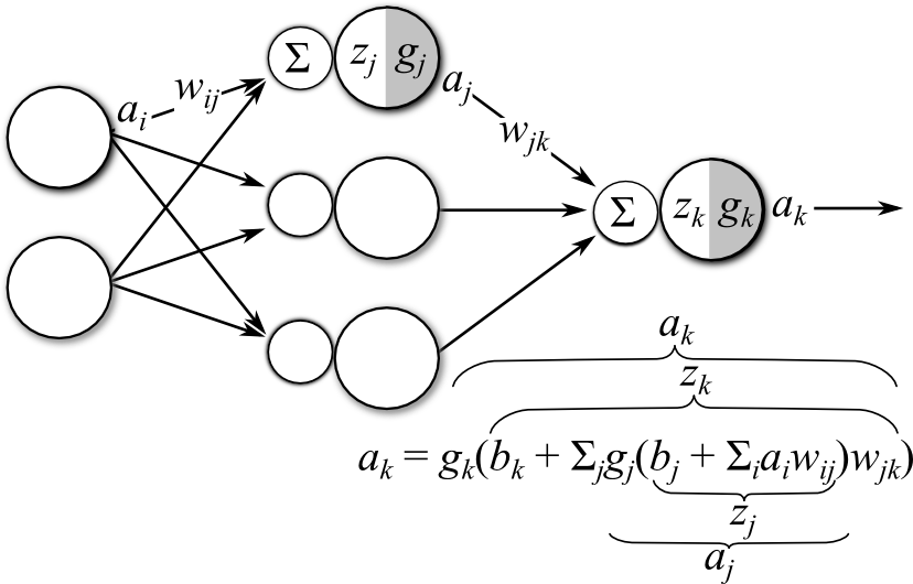
Figure 3: Diagram of a multi-layer ANN. Each node in the network can be considered a single-layered ANN (for simplicity, biases are not visualized in graphical model)
Multi-layer neural networks form compositional functions that map the inputs nonlinearly to outputs. If we associate index \(i\) with the input layer, index \(j\) with the hidden layer, and index \(k\) with the output layer, then an output unit in the network diagrammed in Figure 3 computes an output value \(a_k\) given and input \(a_i\) via the following compositional function:
\[\begin{array}{rcl}a_{\text{out}} = a_k = g_k(b_k + \sum_jg_j(b_j + \sum_i a_i w_{ij})w_{jk}\end{array}\]A breakdown of this function is as follows:
- \(z_l\) is the pre-activation values for the units in layer \(l\)
- \(g_l()\) is the activation function for units in layer \(l\) (assuming the same function for all units)
- \(a_l = g_l(z_l)\) is the output activation for units in layer \(l\).
- \(w_{l-1, l}\) are the parameters that weight the output messages of units feeding into layer \(l\) to the activation function of units for that layer.
- The \(b_l\) term is the bias/DC offset for units in layer \(l\).
As with the single-layered ANN, the choice of activation function for the output layer will depend on the task that we would like the network to perform (i.e. categorization or regression), and follows similar rules outlined above. However, it is generally desirable for the hidden units to have nonlinear activation functions (e.g. logistic sigmoid or tanh). This is because multiple layers of linear computations can be equally formulated as a single layer of linear computations. Thus using linear activations for the hidden layers doesn’t buy us much. However, as we’ll see shortly, using linear activations for the output unit activation function, while in conjunction with nonlinear activations for the hidden units, allows the network to perform nonlinear regression.
Training neural networks & gradient descent
Training neural networks involves determining the model parameters \(\theta = \{\mathbf{w}, \mathbf{b}\}\) that minimize the errors the network makes. This first requires that we have a way of quantifying error. A standard way of quantifying error is to take the squared difference between the network output and the target value:2
\[\begin{array}{rcl}E = \frac{1}{2}(\text{output} - \text{target})^2\end{array}\]With an error function in hand, we then aim to find the setting of parameters that minimizes this error function, when aggregated across all the training data3. This concept can be interpreted spatially by imagining a “parameter space” whose dimensions are the values of each of the model parameters, and for which the error function will form a surface of varying height depending on its value for each parameter. Model training is thus equivalent to finding point in parameter space that makes the height of the error surface small.
Analysis of simple neural networks
Single-layer neural network
To get a better intuition behind the concept of minimizing the error surface, let’s define a super-simple neural network, one that has a single input and a single output. For further simplicity, we’ll assume the network has no bias term and thus has a single parameter, \(w_1\). We will also assume that the output layer uses the logistic sigmoid activation function. Accordingly, the network will map some input value \(a_0\) onto a predicted output \(a_{\text{out}}\) via the following function.
\[\begin{align} a_{\text{out}} &= g_{\text{logistic}}(a_0w_1) \end{align}\]Now let’s say we want this simple network to learn the identity function: given an input of 1 it should return a target value of 1. Given this target value we can now calculate the value of the error function for each setting of \(w_1\). Varying the value of \(w_1\) from -10 to 10 results in the error surface displayed in the right of Figure 4. We see that the error is small for large positive values of \(w_1\), while the error is large for strongly negative values of \(w_1\). This not surprising, given that the output activation function is the logistic sigmoid, which will map large values onto an output of 1.
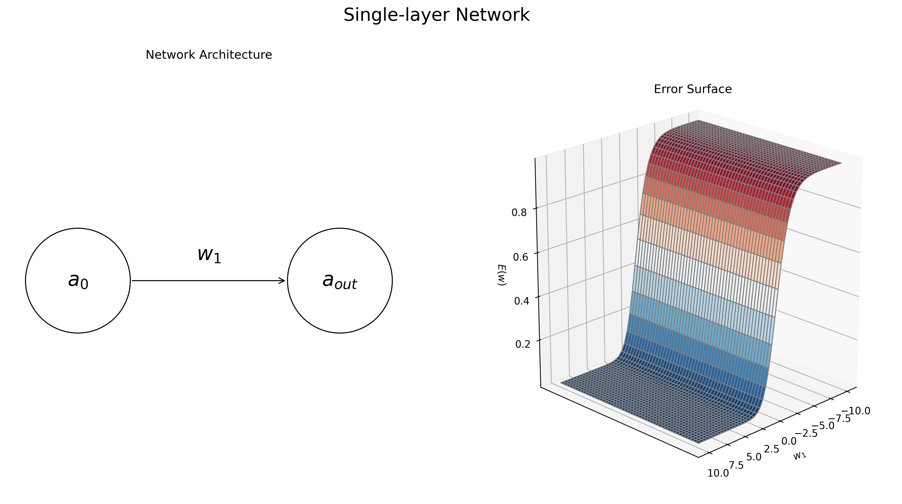
Figure 4: Dynamics of a simple, single-layer neural network. The network’s task is to learn the identity function, i.e. map the input value of 1 to the output value 1. Left: the graphical diagram for the network architecture. Right: the error surface \(E(\mathbf w)\) for the task, as a function of the single model parameter, \(w_1\) The network’s error is low when \(w_1\) large and positive magnitude and high when \(w_1\) is negative
Python Code
from mpl_toolkits.mplot3d import Axes3D
import matplotlib.patches as mpatches

# Sigmoid activation functions
g = g_sigmoid
def error_function(prediction, target):
    """Squared error function (f(x) - y)**2"""
    return (prediction - target)**2

# Grid of allowed parameter values
grid_size = 50
parameter_range = np.linspace(-10, 10, grid_size)
w1, w2 = np.meshgrid(parameter_range, parameter_range)

target_value = 1

# single layer ANN
def single_layer_network_predict(w1, target_value):
    return g(w1 * target_value)


single_layer_network_output = single_layer_network_predict(w1, target_value)
single_layer_network_error = error_function(single_layer_network_output, target_value)

fig = plt.figure(figsize=(16, 8))

ax = fig.add_subplot(1, 2, 1)
input_node = mpatches.Circle((0, .5), 0.1, facecolor='white', edgecolor='black')
output_node = mpatches.Circle((.5, .5), 0.1, facecolor='white', edgecolor='black')
ax.add_patch(input_node)
ax.add_patch(output_node)
ax.text(0, .5, '$a_0$', fontsize=20, ha='center', va='center')
ax.text(.5, .5, '$a_{out}$', fontsize=20, ha='center', va='center')
ax.text(.25, .55, '$w_1$', fontsize=20, ha='center', va='center')

ax.annotate(
    '',
    (.4, .5),
    (.1, .5),
    size=14,
    va="center",
    ha="center",
    arrowprops=dict(
        arrowstyle='->',
        fc="k", ec="k"
    ),
)

plt.xlim([-.25, 1.25])
plt.ylim([0.2, .8])
plt.axis('equal')
plt.axis('off')
plt.title("Network Architecture")

# Plot Error Surface
ERROR_COLORMAP = 'RdBu_r'
edge_color = 'gray'
ax = fig.add_subplot(1, 2, 2, projection='3d')
ax.plot_surface(w1, w2, single_layer_network_error, cmap=ERROR_COLORMAP, edgecolor=edge_color)
plt.yticks([])
ax.view_init(20, 45)
ax.set_xlabel('$w_1$')
ax.set_zlabel('$E(w)$')
plt.title("Error Surface")
plt.suptitle('Single-layer Network', fontsize=18)
Multi-layer neural network
Things become more interesting when we move from a single-layered network to a multi-layered network. Let’s repeat the above exercise, but include a single hidden node between the input and the output. Again, we will assume no biases, and logistic sigmoid activations for both the hidden and output nodes. Thus the network will have two parameters: \((w_1, w_2)\). Accordingly the 2-layered network will predict an output with the following function:
\[\begin{align}a_{\text{out}} &= g_{\text{logistic}}(g_{\text{logistic}}(a_0w_1)w_2)\end{align}\]Now, if we vary both \(w_1\) and \(w_2\), we obtain the error surface in right of Figure 5.
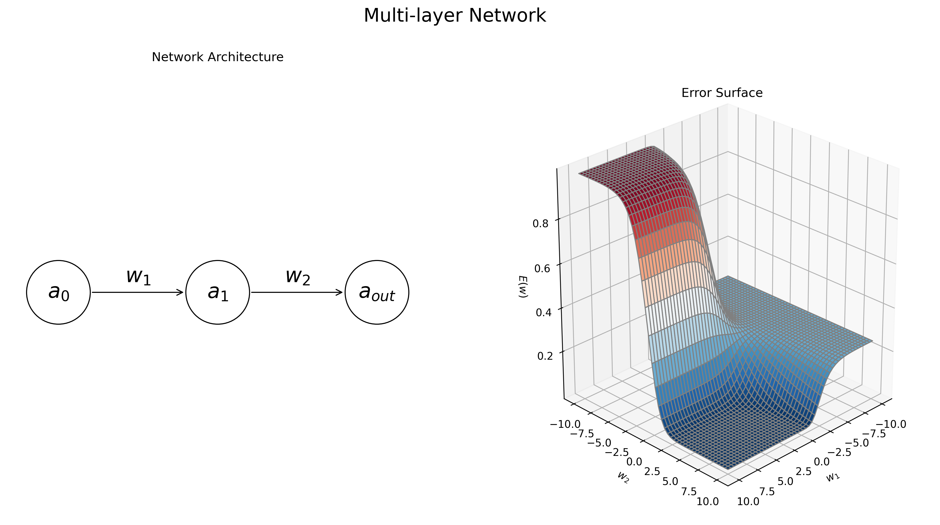
Figure 5: Dynamics of a multi-layer neural network. The network’s task is to learn the identity function, i.e. map the input value of 1 to the output value 1. Left: the graphical diagram for the network architecture. Right: the error surface \(E(\mathbf w)\) for the task, as a function of the model parameters, \(w_1\) and \(w_2\). The network’s error is low when both \(w_1\) and \(w_2\) have large positive magnitudes, and and high when the weights are negative.
Python Code
def two_layer_network_predict(w1, w2, target_value):
    return g(w2 * g(w1 * target_value))

two_layer_network_output = two_layer_network_predict(w1, w2, target_value)
two_layer_network_error = error_function(two_layer_network_output, target_value)

# Plot network diagram
fig = plt.figure(figsize=(16, 8))

ax = fig.add_subplot(1, 2, 1)
input_node = mpatches.Circle((0, .5), 0.1, facecolor='white', edgecolor='black')
hidden_node = mpatches.Circle((.5, .5), 0.1, facecolor='white', edgecolor='black')
output_node = mpatches.Circle((1, .5), 0.1, facecolor='white', edgecolor='black')
ax.add_patch(input_node)
ax.add_patch(hidden_node)
ax.add_patch(output_node)
ax.text(0.0, .5, '$a_0$', fontsize=20, ha='center', va='center')
ax.text(0.5, .5, '$a_1$', fontsize=20, ha='center', va='center')
ax.text(1.0, .5, '$a_{out}$', fontsize=20, ha='center', va='center')

# hidden layer weights
ax.annotate(
    '',
    (.4, .5),
    (.1, .5),
    size=14,
    va="center",
    ha="center",
    arrowprops=dict(
        arrowstyle='->',
        fc="k", ec="k"
    ),
)
ax.text(.25, .55, '$w_1$', fontsize=20, ha='center', va='center')

# output layer weights
ax.annotate(
    '',
    (.6, .5),
    (.9, .5),
    size=14,
    va="center",
    ha="center",
    arrowprops=dict(
        arrowstyle='<-',
        fc="k", ec="k"
    ),
)
ax.text(.75, .55, '$w_2$', fontsize=20, ha='center', va='center')

plt.xlim([-.25, 1.25])
plt.ylim([0.2, .8])
plt.axis('equal')
plt.axis('off')
plt.title("Network Architecture")

# Plot Error Surface
ax = fig.add_subplot(1, 2, 2, projection='3d')
ax.plot_surface(w1, w2, two_layer_network_error, cmap=ERROR_COLORMAP, edgecolor=edge_color)
ax.view_init(25, 45)
ax.set_xlabel('$w_1$')
ax.set_ylabel('$w_2$')
ax.set_zlabel('$E(w)$')
plt.title("Error Surface")
plt.suptitle('Multi-layer Network', fontsize=18)
We see that the error function is minimized when both \(w_1\) and \(w_2\) are large and positive. We also see that the error surface is more complex than for the single-layered model, exhibiting a number of wide plateau regions. It turns out that the error surface gets more and more complicated as you increase the number of layers in the network and the number of units in each hidden layer. Thus, it is important to consider these phenomena when constructing neural network models.
The examples in Figures 4-5 gives us a qualitative idea of how to train the parameters of an ANN, but we would like a more automatic way of doing so. Generally this problem is solved using gradient descent. The gradient descent algorithm first calculates the derivative / gradient of the error function with respect to each of the model parameters. This gradient information will give us the direction in parameter space that decreases the height of the error surface. We then take a step in that direction and repeat, iteratively calculating the gradient and taking steps in parameter space.
The Backpropagation Algorithm
It turns out that the gradient information for the ANN error surface can be calculated efficiently using a message passing algorithm known as the backpropagation algorithm. During backpropagation, input signals are forward-propagated through the network toward the outputs, and network errors are then calculated with respect to target variables and “backpropagated” backwards towards the inputs. The forward and backward signals are then used to determine the direction in the parameter space to move that lowers the network error.
The formal calculations behind the backpropagation algorithm can be somewhat mathematically involved and may detract from the general ideas behind the learning algorithm. For those readers who are interested in the math, I have provided the formal derivation of the backpropagation algorithm (for those of you who are not interested in the math, I would also encourage you go over the derivation and try to make connections to the source code implementations provided later in the post).
Figure 6 demonstrates the four key steps of the backpropagation algorithm. The main concept underlying the algorithm is that for a given observation we want to determine the degree of “responsibility” that each network parameter has for mis-predicting a target value associated with the observation. We then change that parameter according to this responsibility so that it reduces the network error.
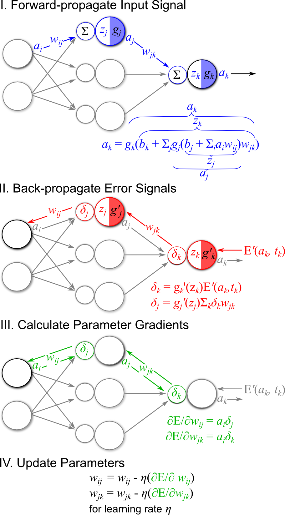
Figure 6: The four key steps of the backpropagation algorithm: I Forward propagate error signals to output, II Calculate output error E, and backpropagate error signal, III Use forward signal and backward signals to calculate parameter gradients, IV update network parameters.
Step I of the backpropagation algorithm is to forward-propagate the observed input forward through the network layers in order to provide a prediction for the current target. This first step of the backpropagation algorithm is demonstrated in Figure 6-I. Note that in the figure \(a_k\) could be considered network output (for a network with one hidden layer) or the output of a hidden layer that projects the remainder of the network (in the case of a network with more than one hidden layer). For this discussion, however, we assume that the index \(k\) is associated with the output layer of the network, and thus each of the network outputs is designated by \(a_k\). Also note that when implementing this forward-propagation step, we should keep track of the feed-forward pre-activations \(z_l\) and activations \(a_l\) for all layers \(l\), as these can be used to efficiently calculate backpropagated errors and error function gradients.
Python Code
def step_I_forwardprop(network_input, weights, biases, g_activation):
    if 'w_2' in weights:  # multi-layer network
        z_hidden = network_input @ weights['w_1'] + biases['b_1']
        a_hidden = g_activation['g_1'](z_hidden)
        z_output = a_hidden @ weights['w_2'] + biases['b_2']
    else:  # single-layer network
        z_hidden = np.array([])
        a_hidden = np.array([])
        z_output = network_input @ weights['w_1'] + biases['b_1']

    a_output = g_activation['g_out'](z_output) # Network prediction
    return a_output, z_output, a_hidden, z_hidden
Step II of the algorithm is to calculate the network output error and backpropagate it toward the input. For this walkthrough we’ll continue to use the sum of squared differences error function, this time written in a more explicit form than in the Training neural networks & gradient descent section:
\[\begin{align}E(\mathbf{\theta}) &= \frac{1}{2}\sum_{k \in K}(a_k - t_k)^2\end{align}\]Here we sum over the values of all \(k\) output units (one in this example). Note that the model parameters parameters \(\theta\) are implicit in the output activations \(a_k\). This error function has the following derivative with respect to the model parameters \(\theta\):
\[E'(\mathbf{\theta}) = (a_k - t_k)\]We can now define an “error signal” \(\delta_k\) at the output node that will be backpropagated toward the input. The error signal is calculated as follows:
\[\begin{align} \delta_k &= g_k'(z_k)E'(\theta) \\ &= g_k'(z_k)(a_k - t_k) \end{align}\]This error signal essentially weights the gradient of the error function by the gradient of the output activation function. Notice that there is a \(z_k\) term is used in the calculation of \(\delta_k\). In order to make learning more efficient, we keep track of the \(z_k\) during the forward-propagation step so that it can be used in backpropagation. We can continue backpropagating the error signal toward the input by passing \(\delta_k\) through the output layer weights \(w_{jk}\), summing over all output nodes, and passing the result through the gradient of the activation function at the hidden layer \(g_j'(z_j)\) (Figure 6-II). Performing these operations results in the backpropagated error signal for the hidden layer, \(\delta_j\):
\[\delta_j = g_j'(z_j)\sum_k \delta_k w_{jk}\]For networks that have more than one hidden layer, this error backpropagation procedure can continue for layers \(j-1, j-2, ...\), etc.
Python Code
def step_II_backprop(target, a_output, z_output, z_hidden, weights, g_activation_prime):
    # Calculate error function derivative given input/output/params
    delta_output = g_activation_prime['g_out'](z_output) * (a_output - target)

    # Calculate any error contributions from hidden layers nodes
    if 'w_2' in weights:  # multi-layer network
        delta_hidden = g_activation_prime['g_1'](z_hidden) * (delta_output @ weights['w_2'].T)
    else:
        delta_hidden = np.array([])
    return delta_output, delta_hidden
Step III of the backpropagation algorithm is to calculate the gradients of the error function with respect to the model parameters at each layer \(l\) using the forward signals \(a_{l-1}\), and the backward error signals \(\delta_l\) . If one considers the model weights \(w_{l-1, l}\) at a layer \(l\) as linking the forward signal \(a_{l-1}\) to the error signal \(\delta_l\) (Figure 6-III), then the gradient of the error function with respect to those weights is:4
\[\frac{\partial E}{\partial w_{l-1, l}} = a_{l-1}\delta_l\]Thus the gradient of the error function with respect to the model weight at each layer can be efficiently calculated by simply keeping track of the forward-propagated activations feeding into that layer from below, and weighting those activations by the backward-propagated error signals feeding into that layer from above!
What about the bias parameters? It turns out that the same gradient rule used for the weight weights applies, except that “feed-forward activations” for biases are always +1 (see Figure 1). Thus the bias gradients for layer \(l\) are simply:
\[\frac{\partial E}{\partial b_{l}} = (1)\delta_l = \delta_l\]Python Code
def step_III_gradient_calculation(
    delta_output, delta_hidden, a_hidden, network_input, weight_gradients, bias_gradients
):
    if 'w_2' in weight_gradients:  # multi-layer network
        weight_gradients['w_2'] = a_hidden.T * delta_output
        bias_gradients['b_2'] = delta_output * 1
        weight_gradients['w_1'] = network_input.T * delta_hidden
        bias_gradients['b_1'] = delta_hidden * 1
    else:  # single-layer network
        weight_gradients['w_1'] = network_input.T * delta_output
        bias_gradients['b_1'] = delta_output * 1

    return weight_gradients, bias_gradients
The fourth and final step of the backpropagation algorithm is to update the model parameters based on the gradients calculated in Step III. Note that the gradients point in the direction in parameter space that will increase the value of the error function. Thus when updating the model parameters we should choose to go in the opposite direction. How far do we travel in that direction? That is generally determined by a user-defined step size–aka learning rate–parameter, \(\eta\). Thus, given the parameter gradients and the step size, the weights and biases for a given layer are updated accordingly:
\[\begin{align} w_{l-1,l} &\leftarrow w_{l-1,l} - \eta \frac{\partial E}{\partial w_{l-1, l}} \\ b_l &\leftarrow b_{l} - \eta \frac{\partial E}{\partial b_{l}} \end{align}\]Python Code
def step_IV_update_parameters(weights, biases, weight_gradients, bias_gradients, learning_rate):
    if 'w_2' in weights:  # multi-layer network
        weights['w_2'] = weights['w_2'] - weight_gradients['w_2'] * learning_rate
        biases['b_2'] = biases['b_2'] - bias_gradients['b_2'] * learning_rate

    weights['w_1'] = weights['w_1'] - weight_gradients['w_1'] * learning_rate
    biases['b_1'] = biases['b_1'] - bias_gradients['b_1'] * learning_rate
    return weights, biases
To train an ANN, the four steps outlined above and in Figure 6 are repeated iteratively by observing many input-target pairs and updating the parameters until either the network error reaches a tolerably low value, the parameters cease to update (convergence), or a set number of iterations over the training data has been achieved. Some readers may find the steps of the backpropagation somewhat ad hoc. However, keep in mind that these steps are formally coupled to the calculus of the optimization problem. Thus I again refer the curious reader to check out the post on deriving the backpropagation algorithm update weight update formulas in order to make connections between the algorithm, the math, and the code, which we’re about to jump into.
Neural Networks for Classification
Here we go over an example of training a single-layered neural network to perform a classification problem. The network is trained to learn a set of logical operators including the AND, OR, or XOR. To train the network we first generate training data. The inputs consist of 2-dimensional coordinates that span the input values \((x_1, x_2)\) values for a 2-bit truth table:
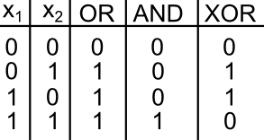
Figure 7: Truth table values learned in classification examples.
We then perturb these observations by adding Normally-distributed noise. To generate target variables, we categorize each observations by applying one of logic operators described in Figure 7) to the original (no-noisy) coordinates.
Python Code
def generate_classification_data(problem_type, n_obs_per_class=30):
    """Generates training data for all demos
    """
    np.random.seed(123)

    truth_table = np.array(
        [
            [0, 0],
            [0, 1],
            [1, 0],
            [1, 1]
        ]
    )

    ring_table = np.vstack(
        [
            truth_table,
            np.array(
                [
                    [.5, .5],
                    [1., .5],
                    [0., .5],
                    [.5, 0.],
                    [.5, 1.]
                ]
            )
        ]
    )
    ring_classes = [1., 1., 1., 1., 0., 1., 1., 1., 1.];

    problem_classes = {
        'AND': np.logical_and(truth_table[:,0], truth_table[:, 1]) * 1.,
        'OR': np.logical_or(truth_table[:,0], truth_table[:, 1]) * 1.,
        'XOR': np.logical_xor(truth_table[:,0], truth_table[:, 1]) * 1.,
        'RING': ring_classes
    }

    if problem_type in ('AND', 'OR', 'XOR'):
        observations = np.tile(truth_table, (n_obs_per_class, 1)) + .15 * np.random.randn(n_obs_per_class * 4, 2)
        obs_classes = np.tile(problem_classes[problem_type], n_obs_per_class)
    else:
        observations = np.tile(ring_table, (n_obs_per_class, 1)) + .15 * np.random.randn(n_obs_per_class * 9, 2)
        obs_classes = np.tile(problem_classes[problem_type], n_obs_per_class)

    # Permute data
    permutation_idx = np.random.permutation(np.arange(len(obs_classes)))
    obs_classes = obs_classes[permutation_idx]
    observations = observations[permutation_idx]
    obs_x = [obs[0] for obs in observations]
    obs_y = [obs[1] for obs in observations]
    return obs_x, obs_y, obs_classes

def generate_regression_data(problem_type='SIN', n_obs=100):
    np.random.seed(123)
    xx = np.linspace(-5, 5, n_obs);
    if problem_type == 'SIN':
        f = lambda x: 2.5 + np.sin(x)
    elif problem_type == 'ABS':
        f = lambda x: abs(x)

    yy = f(xx) + np.random.randn(*xx.shape)*.5
    perm_idx = np.random.permutation(np.arange(n_obs))
    return xx[perm_idx, None], yy[perm_idx]
With training data in hand, we then train the network with the noisy inputs and binary categories targets using the gradient descent / backpropagation algorithm.5
Python Code
from copy import copy

def initialize_network_parameters(n_input_units, n_hidden_units=0, n_output_units=1):
    """Generate weights and bias parameters based on defined network architecture"""
    w1_size = n_hidden_units if n_hidden_units > 0 else n_output_units
    # Weights
    weights = dict()
    weight_gradients = dict()

    weights['w_1'] = np.random.rand(n_input_units, w1_size) - .5
    weight_gradients['w_1'] = np.zeros_like(weights['w_1'])

    if n_hidden_units > 0:
        weights['w_2'] = np.random.rand(n_hidden_units, n_output_units) - .5
        weight_gradients['w_2'] = np.zeros_like(weights['w_2'])

    # Biases
    biases = dict()
    bias_gradients = dict()
    biases['b_1'] = np.random.rand(w1_size) - .5
    bias_gradients['b_1'] = np.zeros_like(biases['b_1'])

    if n_hidden_units > 0:
        biases['b_2'] = np.random.rand(n_output_units) - .5
        bias_gradients['b_2'] = np.zeros_like(biases['b_2'])

    return weights, biases, weight_gradients, bias_gradients

def get_prediction_surface(pred_surface_xy, weights, biases, g_activation):
    """Calculates current prediction surface for classification problem. Used for visualization"""
    prediction_surface = [step_I_forwardprop(xy, weights, biases, g_activation)[0] for xy in pred_surface_xy]
    return np.array(prediction_surface).squeeze().reshape(PREDICTION_SURFACE_RESOLUTION, PREDICTION_SURFACE_RESOLUTION)

def get_prediction_series(pred_x, weights, biases, g_activation):
    """Calculates current prediction series for regression problem. Used for visualization"""
    return step_I_forwardprop(pred_x[:, None], weights, biases, g_activation)[0]

def run_ann_training_simulation(
    problem_type='AND',
    n_hidden_units=0,
    n_iterations=100,
    n_observations=50,
    learning_rate=3
):
    """Simulate ANN training on one of the following problems:

    Binary Classification:
        "AND": noisy binary logical AND data distrubted as 2D datapoints
        "OR": noisy binary logical OR data distrubted as 2D datapoints
        "XOR": noisy binary logical XOR data distrubted as 2D datapoints
        "RING": data are a mode of one binary class surronded by a ring of the other
    Regression (2D)
        "SIN": data are noisy observations around the sin function with a slight vertical offset
        "ABS": data are noisy observations around teh absolute value function

    Parameters
    ----------
    problem_type : str
        One of the problem types listed above
    n_hidden_units : int
        The number of hidden units in the hidden layer. Zero indicates no hidden layer
    n_iterations : int
        The number of times to run through the training observations
    n_observations : int
        The number of data points or (or dataset replicas for classification) that are used
        in the training dataset
    learning_rage : float
        The initial learning rate (annealing is applied at each iteration)

    Returns
    -------
    loss_history : list[float]
        The loss function at each iteration of training
    prediction_history : dict
        Network predictions over the range of the training input. Used for learning visualization.
        Keys are are the iteration number. Values are either prediction surface for classification
        problems, or prediction series for regression
    weights_history : dict
        For each iteration, a snapshot of the state of the parameters. Used for visualizing hidden
        unit states at each iteration
    biases_history : dict
        For each iteration, a snapshot of the state of the biases. Used for visualization. Used for
        visualizing hidden unit states at each iteration
    """

    # Initialize problem data
    if problem_type in ('SIN', 'ABS'):
        observations, targets = generate_regression_data(problem_type, n_observations)
    else:
        obs_x, obs_y, targets = generate_classification_data(problem_type, n_observations)
        observations = np.vstack([obs_x, obs_y]).T

    # Initialize model parameters $\theta$
    n_output_dims = 1
    n_obs, n_input_dims = observations.shape
    weights, biases, weight_gradients, bias_gradients = initialize_network_parameters(
        n_input_dims, n_hidden_units, n_output_dims
    )

    # Initialize problem-specific activation functions and their derivatives
    g_activation = {}
    g_activation_prime = {}
    if problem_type in ('SIN', 'ABS'):  # regression using linear output (and optional tanh hidden) activations
        g_activation['g_out'], g_activation_prime['g_out'], _ = activation_functions['linear']
        if 'w_2' in weights:
            g_activation['g_1'], g_activation_prime['g_1'], _ = activation_functions['tanh']
    else:  # classification using all sigmoid activations
        g_activation['g_out'], g_activation_prime['g_out'], _ = activation_functions['sigmoid']
        if 'w_2' in weights:
            g_activation['g_1'], g_activation_prime['g_1'], _ = activation_functions['sigmoid']

    # Setup for learning history / visualization
    loss_history = []
    prediction_history = {}
    weights_history = {}
    biases_history = {}
    if problem_type in ('SIN', 'ABS'):
        prediction_x = np.linspace(-5, 5, PREDICTION_SURFACE_RESOLUTION)
    else:
        prediction_surface_range = np.linspace(-.5, 1.5, PREDICTION_SURFACE_RESOLUTION)
        prediction_surface_x, prediction_surface_y = np.meshgrid(prediction_surface_range, prediction_surface_range)
        prediction_surface_xy = [(x, y) for x, y in zip(prediction_surface_x.ravel(), prediction_surface_y.ravel())]

    # Run the training
    for iteration in range(n_iterations):
        obs_error = []
        for network_input, target in zip(observations, targets):
            network_input = np.atleast_2d(network_input)

            # Step I: Forward propagate input signal through the network,
            # collecting activations and hidden states
            a_output, z_output, a_hidden, z_hidden = step_I_forwardprop(
                network_input, weights, biases, g_activation
            )

            # Step II: Backpropagate error signal
            delta_output, delta_hidden = step_II_backprop(
                target, a_output, z_output, z_hidden, weights, g_activation_prime
            )

            # Step III. Calculate Error gradient w.r.t. parameters
            weight_gradients, bias_gradients = step_III_gradient_calculation(
                delta_output, delta_hidden, a_hidden, network_input,
                weight_gradients, bias_gradients
            )

            # Step IV. Update model parameters using gradients
            weights, biases = step_IV_update_parameters(
                weights, biases, weight_gradients, bias_gradients, learning_rate
            )

            # Keep track of observation error for loss history
            obs_error.append(error_function(a_output, target))

        # Anneal the learning rate (helps learning)
        learning_rate = learning_rate * .95

        # Keep learning history for visualization
        weights_history[iteration] = copy(weights)
        biases_history[iteration] = copy(biases)
        loss_history.append(sum(obs_error))
        if problem_type in ('SIN', 'ABS'):
            prediction_history[iteration] = get_prediction_series(
                prediction_x, weights, biases, g_activation
            )
        else:
            prediction_history[iteration] = get_prediction_surface(
                prediction_surface_xy, weights, biases, g_activation
            )
    return loss_history, prediction_history, weights_history, biases_history
Below we visualize the progress of the model learning as its trained on the logical OR classification dataset. The code for the classification visualization is here:
Python Code
from matplotlib import pyplot as plt
import matplotlib.animation
from matplotlib.animation import FuncAnimation

PREDICTION_SURFACE_RESOLUTION = 20
PREDICTION_COLORMAP = 'spring'

def visualize_classification_learning(problem_type, loss_history, prediction_history, outfile=None):
    fig, axs = plt.subplots(1, 2, figsize=(12, 6))

    prediction_surface_range = np.linspace(-.5, 1.5, PREDICTION_SURFACE_RESOLUTION)
    prediction_surface_x, prediction_surface_y = np.meshgrid(prediction_surface_range, prediction_surface_range)

    xx, yy, cls = generate_classification_data(problem_type=problem_type)

    # Initialize plots
    contour = axs[0].contourf(
        prediction_surface_x,
        prediction_surface_y,
        prediction_history[0]
    )
    points = axs[0].scatter(xx, yy, c=cls, cmap='gray_r')
    axs[0].set_title("Prediction Surface")
    line = axs[1].plot(loss_history[0], 'r-', linewidth=2)[0]
    axs[1].set_title("Loss Function")
    suptitle = plt.suptitle("Iteration: 0", fontsize=16)

    def animate(ii):
        plt.suptitle("Iteration: {}".format(ii + 1), fontsize=16)
        axs[0].clear()
        contour = axs[0].contourf(
            prediction_surface_x,
            prediction_surface_y,
            prediction_history[ii]
        )
        axs[0].scatter(xx, yy, c=cls, cmap='gray_r')
        axs[0].set_title("Prediction Surface")
        line = axs[1].plot(loss_history[:ii], 'r-', linewidth=2)
        axs[1].set_title("Loss Function")
        return axs, contour, line

    anim = FuncAnimation(
        fig,
        animate,
        frames=np.arange(len(loss_history)),
        interval=50, repeat=False
    )
    plt.show()
    if outfile:
        # anim.save requires imagemagick library to be installed
        anim.save(outfile, dpi=80, writer='imagemagick')
Figure 8: Learning the logical OR function using a single-layer ANN (aka “perceptron”). Network architecture includes a single sigmoid output encoding the class. (Left) The colormap indicates the probability that a location in the 2D map will be associated with a positive (black) or negative class (white). Because the classes can be separated with a linear decision function, the single layer network is able to classify the points with low error (right).
Python Code
N_HIDDEN_UNITS = 0
PROBLEM_TYPE = 'OR'
loss_history, prediction_history, _, _ = run_ann_training_simulation(
    problem_type=PROBLEM_TYPE,
    n_hidden_units=N_HIDDEN_UNITS,
    n_iterations=100,
    learning_rate=2,
)

visualize_classification_learning(
    PROBLEM_TYPE,
    loss_history,
    prediction_history
)
Figure 8 displays the network state when learning the OR mapping. The left plot displays the training data and the network output at each iteration. Black dots are training points categorized 1 while white dots are categorized 0. Blue regions are where the network predicts values of 0, while green highlights areas where the network predicts 1. We see that the single-layer network is able to easily separate the two classes. The right plot shows how the loss function (the total error over all training observations) decreases with each training iteration.
Figure 9: Learning the logical AND function using a single-layer ANN. Network architecture includes a single sigmoid output encoding the binary class. (Left) The colormap indicates the probability that a location in the 2D map will be associated with a positive (black) or negative class (white). Because the classes can be separated with a linear decision function, the single layer network is able to classify the points with low error (right).
Python Code
N_HIDDEN_UNITS = 0
PROBLEM_TYPE = 'AND'
loss_history, prediction_history, _, _ = run_ann_training_simulation(
    problem_type=PROBLEM_TYPE,
    n_hidden_units=N_HIDDEN_UNITS,
    n_iterations=100,
    learning_rate=2,
)

visualize_classification_learning(
    PROBLEM_TYPE,
    loss_history,
    prediction_history
)
Figure 9 demonstrates an analogous example, but instead learning the logical AND operator. Again, the categories can be easily separated by a linear decision boundary (i.e. a plane), and thus the single-layered network easily learns an accurate predictor of the data, as indicated by the small loss function value after a number of iterations.
Going Deeper: Nonlinear classification and multi-layer neural networks
Figures 8 and 9 demonstrate how a single-layered ANN can easily learn the OR and AND operators. This is because the decision function required to represent these logical operators is a single linear function (i.e. line/plane) of the input space. What about more complex categorization criterion that cannot be represented by a single plane? An example of a more complex binary classification criterion is the XOR operator (Figure 7, far right column).
Below we attempt to train the single-layer network to learn the XOR operator. The single layer network is unable to learn this nonlinear mapping between the inputs and the targets. However, it turns out we can learn the XOR operator using a multi-layered neural network.
Figure 10: Learning the logical XOR function using a single-layer ANN. Network architecture includes a single sigmoid output encoding the binary class. (Left) The colormap indicates the probability that a location in the 2D map will be associated with a positive (black) or negative class (white). Because the classes can be cannot be separated with a linear decision function, the single layer network is unable to classify the points accurately (right).
Python Code
N_HIDDEN_UNITS = 0
PROBLEM_TYPE = 'XOR'
loss_history, prediction_history, _, _ = run_ann_training_simulation(
    problem_type=PROBLEM_TYPE,
    n_hidden_units=N_HIDDEN_UNITS,
    n_iterations=100,
    learning_rate=2,
)

visualize_classification_learning(
    PROBLEM_TYPE,
    loss_history,
    prediction_history
)
Below we instead train a two-layer (i.e. single-hidden-layer) neural network on the XOR dataset. The network incorporates a hidden layer with 4 hidden units and logistic sigmoid activation functions for all units in the hidden and output layers.
Figure 11: Learning the logical XOR function using a multi-layer ANN. Network architecture includes a hidden layer with 4 sigmoid units and a single sigmoid output unit encoding the binary class. (Left) The colormap indicates the probability that a location in the 2D map will be associated with a positive (black) or negative class (white). The multi-layer network is able to capture a linear decision function, and is thus able to classify the points accurately (right).
Python Code
N_HIDDEN_UNITS = 4
PROBLEM_TYPE = 'XOR'
loss_history, prediction_history, _, _ = run_ann_training_simulation(
    problem_type=PROBLEM_TYPE,
    n_hidden_units=N_HIDDEN_UNITS,
    n_iterations=100,
    learning_rate=2,
)

visualize_classification_learning(
    PROBLEM_TYPE,
    loss_history,
    prediction_history
)
Figure 11 displays the learning process for the 2-layer network on the XOR dataset. The 2-layer network is easily able to learn the XOR operator. We see that by adding a hidden layer between the input and output, the ANN is able to learn the nonlinear categorization criterion!
Figure 12 shows the results for learning a even more difficult nonlinear categorization function: points in and around \((x1, x2) = (0.5, 0.5)\) are categorized as 1, while points in a ring surrounding the 1 datapoints are categorized as a 0:
Figure 12: Nonlinear classification using a multi-layer ANN. Network architecture includes a hidden layer with 4 sigmoid units, and a single sigmoid output encoding the class. Colormap indicates the probability that an area in the 2D map will be associated with a positive (black) or negative (white) class.
Python Code
N_HIDDEN_UNITS = 4
PROBLEM_TYPE = 'RING'
loss_history, prediction_history, _, _ = run_ann_training_simulation(
    problem_type=PROBLEM_TYPE,
    n_hidden_units=N_HIDDEN_UNITS,
    n_iterations=100,
    learning_rate=2,
)

visualize_classification_learning(
    PROBLEM_TYPE,
    loss_history,
    prediction_history
)
Figure 12 visualizes the learning process on the RING dataset. The 2-layer ANN is able to easily learn this difficult classification criterion in a 40 iterations or so.
Neural Networks for Regression
The previous examples demonstrated how ANNs can be used for classification by using a logistic sigmoid as the output activation function. Here we demonstrate how, by making the output activation function the linear/identity function, the same 2-layer network architecture can be used to implement nonlinear regression.
For this example we define a dataset comprised of 1D inputs, \(\mathbf{x}\) that range from \((-5, 5)\). We then generate noisy targets \(\mathbf y\) according to the function:
\[\mathbf{y} = f(\mathbf{x}) + \mathbf{\epsilon}\]where \(f(\mathbf{x})\) is a nonlinear data-generating function and \(\mathbf \epsilon\) is Normally-distributed noise. We then construct a two-layered network with \(\text{tanh}\) activation functions used in the hidden layer and linear outputs. For this example we set the number of hidden units to 3 and train the model as we did for categorization using gradient descent / backpropagation. The results of the example are visualized below.
Python Code
def visualize_regression_learning(problem_type, loss_history, prediction_history, weights_history, biases_history, outfile=None):
    fig, axs = plt.subplots(1,2, figsize=(12, 8))

    prediction_surface_range = np.linspace(-.5, 1.5, PREDICTION_SURFACE_RESOLUTION)
    prediction_surface_x, prediction_surface_y = np.meshgrid(prediction_surface_range, prediction_surface_range)

    xx, yy = generate_regression_data(problem_type=problem_type, n_obs=len(prediction_history[0]))
    pred_xx = np.linspace(-5, 5, PREDICTION_SURFACE_RESOLUTION)

    def get_hidden_unit_predictions(pred_xx, weights, biases):
        return g_tanh(pred_xx[:, None] @ weights['w_1'] + biases['b_1']) * weights['w_2'].T + biases['b_2']

    # Initialize plots
    points = axs[0].scatter(xx, yy, marker='o', c='magenta', label='Data')
    ii = 0
    pred_line = axs[0].plot(pred_xx, prediction_history[ii], c='blue', label='Network Prediction')
    hidden_predictions = get_hidden_unit_predictions(pred_xx, weights_history[ii], biases_history[ii])

    for hj, hidden_pred in enumerate(hidden_predictions.T):
        axs[0].plot(pred_xx, hidden_pred, '--', label=f'$a_^{(1)}w_ + b_{k}$')

    axs[0].set_title("Data and Prediction")
    axs[0].legend(loc='upper left')
    loss_line = axs[1].plot(loss_history[:ii], 'r-', linewidth=2)
    axs[1].set_title("Loss Function")
    suptitle = fig.suptitle(f"Iteration: {ii}", fontsize=16)

    def animate(ii):
        suptitle = fig.suptitle("Iteration: {}".format(ii + 1), fontsize=16)
        axs[0].clear()
        points = axs[0].scatter(xx, yy, marker='o', c='magenta', label='Data')
        pred_line = axs[0].plot(pred_xx, prediction_history[ii], c='blue', label='Network Prediction')
        hidden_predictions = get_hidden_unit_predictions(pred_xx, weights_history[ii], biases_history[ii])

        for hj, hidden_pred in enumerate(hidden_predictions.T):
            axs[0].plot(pred_xx, hidden_pred, '--', label=f'$a_^{(1)}w_ + b_{k}$')

        axs[0].set_title("Data and Prediction")
        axs[0].legend(loc='upper left')
        loss_line = axs[1].plot(loss_history[:ii+1], 'r-', linewidth=2)
        axs[1].set_title("Loss Function")

        return axs, pred_line, loss_line, suptitle

    anim = FuncAnimation(
        fig,
        animate,
        frames=np.arange(len(loss_history)),
        interval=50, repeat=False
    )
    plt.show()

    if outfile:
        anim.save(outfile, dpi=80, writer='imagemagick')
Figure 13: Nonlinear regression using a multi-layer ANN. The task is to learn the noisy sin function with an additional vertical offset (magenta datapoints). Network architecture includes a hidden layer with 3 tanh units, and a single linear output unit. (Left subpanel) The weighted hidden unit outputs \(a_{j}^{(1)}w_{jk} + b_k\) that are combined to form the network prediction (in blue) are plotted as dashed lines, where we use the notation \(a^{(l)}\) to indicate activations in the \(l\)-th hidden layer.
Python Code
N_HIDDEN_UNITS = 3
PROBLEM_TYPE = 'SIN'
loss_history, prediction_history, weights_history, biases_history = run_ann_simulation(
    problem_type=PROBLEM_TYPE,
    n_hidden_units=N_HIDDEN_UNITS,
    n_observations=200,
    n_iterations=100,
    learning_rate=.2,
)

visualize_regression_learning(
    PROBLEM_TYPE,
    loss_history,
    prediction_history,
    weights_history,
    biases_history
)
The training procedure for \(f(x): \sin(x) + 2.5\) is visualized in the left plot of Figure 13. Noisy data generated around the function \(f(x)\) are plotted in magenta. The output of the network at each training iteration is plotted in solid blue while the output of each of the tanh hidden units is plotted in dashed lines. This visualization demonstrates how multiple nonlinear functions are combined by the ANN to form the complex output target function. The total squared error loss at each iteration is plotted in the right plot of Figure 13.
Figure 14 visualizes the training procedure for trying to learn a different nonlinear function, namely \(f(x): \text{abs}(x)\). Again, we see how the outputs of the hidden units are combined to fit the desired data-generating function. The total squared error loss again follows an erratic path during learning.
Figure 14: Nonlinear regression using a multi-layer ANN. The task is to learn the noisy abs function (magenta datapoints). Network architecture includes a hidden layer with 3 tanh units, and a single linear output unit. (Left subpanel) The weighted hidden unit outputs \(a_{j}^{(1)}w_{jk} + b_k\) that are combined to form the network prediction (in blue) are plotted as dashed lines, where we use the notation \(a^{(l)}\) to indicate activations in the \(l\)-th hidden layer..
Python Code
N_HIDDEN_UNITS = 3
PROBLEM_TYPE = 'ABS'
loss_history, prediction_history, weights_history, biases_history = run_ann_simulation(
    problem_type=PROBLEM_TYPE,
    n_hidden_units=N_HIDDEN_UNITS,
    n_observations=200,
    n_iterations=100,
    learning_rate=.2,
)

visualize_regression_learning(
    PROBLEM_TYPE,
    loss_history,
    prediction_history,
    weights_history,
    biases_history
)
Wrapping up
In this post we covered the main ideas behind artificial neural networks including: single- and multi-layer ANNs, activation functions and their derivatives, a high-level description of the backpropagation algorithm, and a number of classification and regression examples. ANNs, particularly multi-layer ANNs, are a robust and powerful class of models that can be used to learn complex, nonlinear functions. However, there are a number of considerations when using neural networks including:
- How many hidden layers should one use?
- How many hidden units in each layer?
- How do these relate to overfitting and generalization?
- Are there better error functions than the squared difference?
- What should the learning rate be?
- What can we do about the complexity of error surface with deep networks?
- Should we use simulated annealing?
- What about other activation functions?
It turns out that there are no easy or definite answers to any of these questions, and there is active research focusing on each topic. This is why using ANNs is often considered as much as a “black art” as it is a quantitative technique.
One primary limitation of ANNs is that they are supervised algorithms, requiring a target value for each input observation in order to train the network. This can be prohibitive for training large networks that may require lots of training data to adequately adjust the parameters. However, there are a set of unsupervised variants of ANNs that can be used to learn an initial condition for the ANN (rather than from randomly-generated initial weights) without the need of target values. This technique of “unsupervised pretraining” has been an important component of many “deep learning” models used in AI and machine learning. In future posts, I look forward to covering two of these unsupervised neural networks: autoencoders and restricted Boltzmann machines.
Notes
This post is a refactor of content with the same title originally posted on The Clever Machine Wordpress blog.
-
This property is not reserved for ANNs; kernel methods are also considered “universal approximators”; however, it turns out that neural networks with multiple layers are more efficient at approximating arbitrary functions than other methods. I refer the interested reader to an in-depth discussion on the topic.) ↩
-
The squared error is not chosen arbitrarily, but has a number of theoretical benefits and considerations. For more detail, see the this post on the matter ↩
-
Aggregating the error across all training observations yields a loss function, which we discuss in depth in this post ↩
-
Note that this result is closely related to the concept of Hebbian learning in neuroscience ↩
-
Notice for the implementation, there is an additional step known as learning rate annealing. This technique decreases the learning rate after every iteration thus making the algorithm take smaller and smaller steps in parameter space. This technique can be useful when the gradient updates begin oscillating between two or more locations in the parameter space. It is also helpful for influencing the algorithm to settle down into a steady state. ↩