Tanveer Khan Data Scientist @ NextGen Invent | Research Scholar @ Jamia Millia Islamia
CNN for handwritten digit recognition problem on MNIST dataset
Convolutional Neural Networks (CNNs) are the current state-of-art architecture for image classification task. Whether it is facial recognition, self driving cars or object detection, CNNs are being used everywhere. In this post, a simple 2-D Convolutional Neural Network (CNN) model is designed using keras with tensorflow backend for the well known MNIST digit recognition task. The whole work flow can be described as:
- 1. Preparing the data
- 2. Building and compiling of the model
- 3. Training and evaluating the model
- 4. Saving the model to disk for reuse
Preparing the data
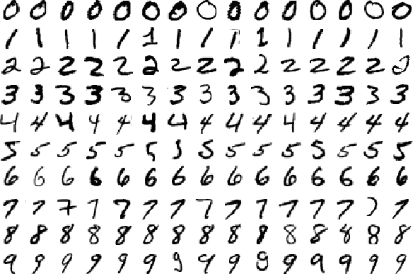
The data set used here is MNIST dataset as mentioned above. The MNIST database (Modified National Institute of Standards and Technology database) is a large database of handwritten digits (0 to 9). The database contains 60,000 training images and 10,000 testing images each of size 28x28. The first step is to load the dataset, which can be easily done through the keras api.
  import keras
  from keras.datasets import mnist
  #load mnist dataset
  (X_train, y_train), (X_test, y_test) = mnist.load_data() #everytime loading data won't be so easy :)
Here X_train contains 60,000 training images’ data each of size 28x28 and y_train contains their corresponding labels. Similarly, X_test contains 10,000 testing images’ data each of dimension 28x28 and y_test contains their corresponding labels. Let’s visualize few data from training to get a better idea about the purpose of the deep learning model.
  import matplotlib.pyplot as plt
  fig = plt.figure()
  for i in range(9):
    plt.subplot(3,3,i+1)
    plt.tight_layout()
    plt.imshow(X_train[i], cmap='gray', interpolation='none')
    plt.title("Digit: {}".format(y_train[i]))
    plt.xticks([])
    plt.yticks([])
  fig
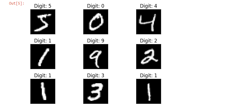
As can be seen here, at left top corner the image of ‘5’ is stored is X_train[0] and y_train[0] contains label ‘5’. Our deep learning model should be able to only take the handwritten image and predict the actual digit written.
Now, to prepare the data we need some processing on the images like resizing images, normalizing the pixel values etc.
#reshaping
#this assumes our data format
#For 3D data, "channels_last" assumes (conv_dim1, conv_dim2, conv_dim3, channels) while
#"channels_first" assumes (channels, conv_dim1, conv_dim2, conv_dim3).
if k.image_data_format() == 'channels_first':
    X_train = X_train.reshape(X_train.shape[0], 1, img_rows, img_cols)
    X_test = X_test.reshape(X_test.shape[0], 1, img_rows, img_cols)
    input_shape = (1, img_rows, img_cols)
else:
    X_train = X_train.reshape(X_train.shape[0], img_rows, img_cols, 1)
    X_test = X_test.reshape(X_test.shape[0], img_rows, img_cols, 1)
    input_shape = (img_rows, img_cols, 1)
#more reshaping
X_train = X_train.astype('float32')
X_test = X_test.astype('float32')
X_train /= 255
X_test /= 255
print('X_train shape:', X_train.shape) #X_train shape: (60000, 28, 28, 1)
After doing the necessary processing on the image informations, the label data i.e. y_train and y_test need to be converted into categorical formats like label ‘3’ should be converted to a vector [0, 0, 0, 1, 0, 0, 0, 0, 0, 0] for model building.
import keras
#set number of categories
num_category = 10
# convert class vectors to binary class matrices
y_train = keras.utils.to_categorical(y_train, num_category)
y_test = keras.utils.to_categorical(y_test, num_category)
Building and compiling of the model
After the data is ready to be fed to the model, we need to define the architecture of the model and compile it with necessary optimizer function, loss function and performance metrics.
The architecture followed here is 2 convolution layers followed by pooling layer, a fully connected layer and softmax layer respectively. Multiple filters are used at each convolution layer, for different types of feature extraction. One intuitive explanation can be if first filter helps in detecting the straight lines in the image, second filter will help in detecting circles and so on.
After both maxpooling and fully connected layer, dropout is introduced as regularization in our model to reduce over-fitting problem.
##model building
model = Sequential()
#convolutional layer with rectified linear unit activation
model.add(Conv2D(32, kernel_size=(3, 3),
                 activation='relu',
                 input_shape=input_shape))
#32 convolution filters used each of size 3x3
#again
model.add(Conv2D(64, (3, 3), activation='relu'))
#64 convolution filters used each of size 3x3
#choose the best features via pooling
model.add(MaxPooling2D(pool_size=(2, 2)))
#randomly turn neurons on and off to improve convergence
model.add(Dropout(0.25))
#flatten since too many dimensions, we only want a classification output
model.add(Flatten())
#fully connected to get all relevant data
model.add(Dense(128, activation='relu'))
#one more dropout for convergence' sake :)
model.add(Dropout(0.5))
#output a softmax to squash the matrix into output probabilities
model.add(Dense(num_category, activation='softmax'))
After the architecture of the model is defined, the model needs to be compiled. Here, we are using categorical_crossentropy loss function as it is a multi-class classification problem. Since all the labels carry similar weight we prefer accuracy as performance metric. A popular gradient descent technique called AdaDelta is used for optimization of the model parameters.
#Adaptive learning rate (adaDelta) is a popular form of gradient descent rivaled only by adam and adagrad
#categorical ce since we have multiple classes (10)
model.compile(loss=keras.losses.categorical_crossentropy,
              optimizer=keras.optimizers.Adadelta(),
              metrics=['accuracy'])
Training and evaluating the model
After the model architecture is defined and compiled, the model needs to be trained with training data to be able to recognize the handwritten digits. Hence we will fit the model with X_train and y_train.
batch_size = 128
num_epoch = 10
#model training
model_log = model.fit(X_train, y_train,
          batch_size=batch_size,
          epochs=num_epoch,
          verbose=1,
          validation_data=(X_test, y_test))
Here, one epoch means one forward and one backward pass of all the training samples. Batch size implies number of training samples in one forward/backward pass.
Now the trained model needs to be evaluated in terms of performance.
score = model.evaluate(X_test, y_test, verbose=0)
print('Test loss:', score[0]) #Test loss: 0.0296396646054
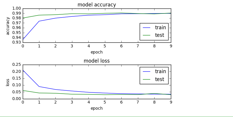
print('Test accuracy:', score[1]) #Test accuracy: 0.9904
Test accuracy 99%+ implies the model is trained well for prediction. If we visualize the whole training log, then with more number of epochs the loss and accuracy of the model on training and testing data converged thus making the model a stable one.
import os
# plotting the metrics
fig = plt.figure()
plt.subplot(2,1,1)
plt.plot(model_log.history['acc'])
plt.plot(model_log.history['val_acc'])
plt.title('model accuracy')
plt.ylabel('accuracy')
plt.xlabel('epoch')
plt.legend(['train', 'test'], loc='lower right')
plt.subplot(2,1,2)
plt.plot(model_log.history['loss'])
plt.plot(model_log.history['val_loss'])
plt.title('model loss')
plt.ylabel('loss')
plt.xlabel('epoch')
plt.legend(['train', 'test'], loc='upper right')
plt.tight_layout()
fig
Saving the model to disk for reuse
Now, the trained model needs to be serialized. The architecture or structure of the model will be stored in a json file and the weights will be stored in hdf5 file format.
#Save the model
# serialize model to JSON
model_digit_json = model.to_json()
with open("model_digit.json", "w") as json_file:
    json_file.write(model_digit_json)
# serialize weights to HDF5
model.save_weights("model_digit.h5")
print("Saved model to disk")
Hence the saved model can be reused later or easily ported to other environments too.
References
- Ahlawat, S., Choudhary, A., Nayyar, A., Singh, S., & Yoon, B. (2020). Improved handwritten digit recognition using convolutional neural networks (CNN). Sensors, 20(12), 3344.
- Teow, M. Y. (2017, October). A minimal convolutional neural network for handwritten digit recognition. In 2017 7th IEEE International Conference on System Engineering and Technology (ICSET) (pp. 171-176). IEEE.