Convolutional Neural Network based Breast Cancer Classification

Breast cancer is the second most common cancer worldwide. In 2012, it represented about 12 percent of all new cancer cases and 25 percent of all cancers in women.

Breast cancer starts when cells in the breast begin to grow out of control. These cells usually form a tumor that can often be seen on an x-ray or felt as a lump. The tumor is malignant (cancer) if the cells can grow into (invade) surrounding tissues or spread (metastasize) to distant areas of the body.

The Objective

To design an algorithm to automatically identify whether a patient is suffering from breast cancer or not by analysing the histology images.

Dataset

Breast histopathology images can be downloaded from Kaggle’s website.. The data consists of 227, 524 patches of 50 x 50 pixels which was extracted from 162 whole mount slide images of Breast Cancer specimens scanned at 40x. The data contains images of both negative and positive examples where the number of of positive examples are over two times less than negative examples (classic case of imbalanced data):

Negative Examples (No Cancer — benign): 198, 738

Positive Examples (Cancer — malignant): 78, 786

Prepare the Data for Model Training, Validation and Testing.

In this section, we will segment our dataset into train, validation and test sets. As indicated earlier, there are around 227, 524 images out of which 38, 000 images will be used for validation and another 38, 000 images for testing purpose. The remaining 201, 524 images will be used for training the model. Here is the break down:

Train: 201, 524 images
Validation: 38, 000 images
Test: 38, 000 images

CNN Architecture

Let’s go step by step and analyze each layer in the Convolutional Neural Network.

Input

A Matrix of pixel values in the shape of [WIDTH, HEIGHT, CHANNELS]. Let’s assume that our input is [32x32x3].

Convolution

The purpose of this layer is to receive a feature map. Usually, we start with low number of filters for low-level feature detection. The deeper we go into the CNN, the more filters we use to detect high-level features. Feature detection is based on ‘scanning’ the input with the filter of a given size and applying matrix computations in order to derive a feature map.

Pooling

The goal of this layer is to provide spatial variance, which simply means that the system will be capable of recognizing an object even when its appearance varies in some way. Pooling layer will perform a downsampling operation along the spatial dimensions (width, height), resulting in output such as [16x16x12] for pooling_size=(2, 2).

Fully Connected

In a fully connected layer, we flatten the output of the last convolution layer and connect every node of the current layer with the other nodes of the next layer. Neurons in a fully connected layer have full connections to all activations in the previous layer, as seen in regular Neural Networks and work in a similar way.

Image Classification

The complete image classification pipeline can be formalized as follows: Our input is a training dataset that consists of N images, each labeled with one of the 2 different classes.

Then, we use this training set to train a classifier to learn what every one of these histology images belongs to i.e. benign or malignant. In the end, we evaluate the performance of the classifier by using it to predict labels for a new set of images that it has never seen before. We will then compare the true labels of these images to the ones predicted by the classifier. Furthermore, the obatained results are reported in terms of standard metrics.

Let's begin our deep learning model building...!!!!

Let’s start with loading all the libraries and dependencies.

Loading Packages



import json
import math
import os
import cv2
from PIL import Image
import numpy as np
from keras import layers
from keras.applications import DenseNet201
from keras.callbacks import Callback, ModelCheckpoint, ReduceLROnPlateau, TensorBoard
from keras.preprocessing.image import ImageDataGenerator
from keras.utils.np_utils import to_categorical
from keras.models import Sequential
from keras.optimizers import Adam
import matplotlib.pyplot as plt
import pandas as pd
from sklearn.model_selection import train_test_split
from sklearn.metrics import cohen_kappa_score, accuracy_score
import scipy
from tqdm import tqdm
import tensorflow as tf
from keras import backend as K
import gc
from functools import partial
from sklearn import metrics
from collections import Counter
import json
import itertools

Laoding the dataset

Loading the images.



def Dataset_loader(DIR, RESIZE, sigmaX=10):
  IMG = []
  read = lambda imname: np.asarray(Image.open(imname).convert("RGB"))
  for IMAGE_NAME in tqdm(os.listdir(DIR)):
      PATH = os.path.join(DIR,IMAGE_NAME)
      _, ftype = os.path.splitext(PATH)
      if ftype == ".png":
          img = read(PATH)

          img = cv2.resize(img, (RESIZE,RESIZE))

          IMG.append(np.array(img))
 return IMG

benign_train = np.array(Dataset_loader('data/train/benign',224))
malign_train = np.array(Dataset_loader('data/train/malignant',224))
benign_test = np.array(Dataset_loader('data/validation/benign',224))
malign_test = np.array(Dataset_loader('data/validation/malignant',224))

After loading of the histology images we will create a numpy array of zeroes for labeling "benign" and "malgnant" images and then shuffling the dataset for converting the labels into a categorical format.



  benign_train_label = np.zeros(len(benign_train))
  malign_train_label = np.ones(len(malign_train))
  benign_test_label = np.zeros(len(benign_test))
  malign_test_label = np.ones(len(malign_test))

  X_train = np.concatenate((benign_train, malign_train), axis = 0)
  Y_train = np.concatenate((benign_train_label, malign_train_label), axis = 0)
  X_test = np.concatenate((benign_test, malign_test), axis = 0)
  Y_test = np.concatenate((benign_test_label, malign_test_label), axis = 0)

  s = np.arange(X_train.shape[0])
  np.random.shuffle(s)
  X_train = X_train[s]
  Y_train = Y_train[s]

  s = np.arange(X_test.shape[0])
  np.random.shuffle(s)
  X_test = X_test[s]
  Y_test = Y_test[s]

  Y_train = to_categorical(Y_train, num_classes= 2)
  Y_test = to_categorical(Y_test, num_classes= 2))

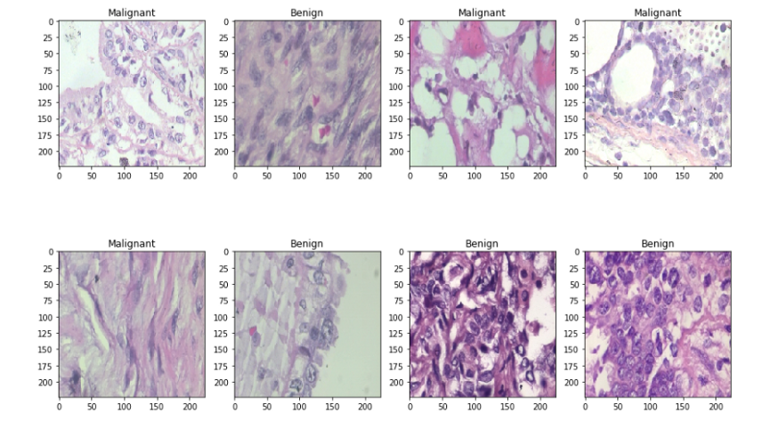
We will split the dataset into two sets — train and test sets with 80% and 20% images respectively. Let’s see some sample benign and malignant images.



  x_train, x_val, y_train, y_val = train_test_split(
      X_train, Y_train,
      test_size=0.2,
      random_state=11
  )

  w=60
  h=40
  fig=plt.figure(figsize=(15, 15))
  columns = 4
  rows = 3

  for i in range(1, columns*rows +1):
      ax = fig.add_subplot(rows, columns, i)
      if np.argmax(Y_train[i]) == 0:
          ax.title.set_text('Benign')
      else:
          ax.title.set_text('Malignant')
      plt.imshow(x_train[i], interpolation='nearest')
  plt.show()

brstimag

CNN model building

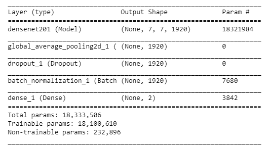
We will use the "DenseNet201" as the pre trained weights which is already trained on the Imagenet datset with a learning rate of 0.0001. Furthermore, globalaveragepooling layer followed by 50% dropouts to reduce over-fitting. Using batch normalization and a dense layer with 2 neurons for 2 output classes i.e. "benign" and "malignant" with softmax as the activation function and Adam as the optimizer and binary-cross-entropy as the loss function.



  def build_model(backbone, lr=1e-4):
      model = Sequential()
      model.add(backbone)
      model.add(layers.GlobalAveragePooling2D())
      model.add(layers.Dropout(0.5))
      model.add(layers.BatchNormalization())
      model.add(layers.Dense(2, activation='softmax'))

      model.compile(
          loss='binary_crossentropy',
          optimizer=Adam(lr=lr),
          metrics=['accuracy']
      )
      return model

  resnet = DenseNet201(
      weights='imagenet',
      include_top=False,
      input_shape=(224,224,3)
  )

  model = build_model(resnet ,lr = 1e-4)
  model.summary()

Let’s look at the output shape and the parameters involved in each layer.

mdlsummry

CNN model training

Before training of the model, it is useful to define one or more callbacks. some useful one's are: ModelCheckpoint and ReduceLROnPlateau.



  learn_control = ReduceLROnPlateau(monitor='val_acc', patience=5,
                                  verbose=1,factor=0.2, min_lr=1e-7)

filepath="weights.best.hdf5"
checkpoint = ModelCheckpoint(filepath, monitor='val_acc', verbose=1, save_best_only=True, mode='max')

history = model.fit_generator(
    train_generator.flow(x_train, y_train, batch_size=BATCH_SIZE),
    steps_per_epoch=x_train.shape[0] / BATCH_SIZE,
    epochs=20,
    validation_data=(x_val, y_val),
    callbacks=[learn_control, checkpoint])

Model performance evaluation

The most common metric for evaluating model performance is the accurcacy. However, when only 2% of your dataset is of one class (malignant) and 98% some other class (benign), misclassification scores don’t really make sense. You can be 98% accurate and still catch none of the malignant cases which could make a terrible classifier.



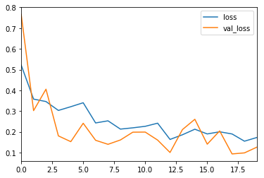
  history_df = pd.DataFrame(history.history)
  history_df[['loss', 'val_loss']].plot()

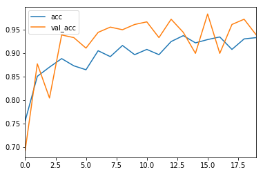
  history_df = pd.DataFrame(history.history)
  history_df[['acc', 'val_acc']].plot()

lssvsepch

accvsepch

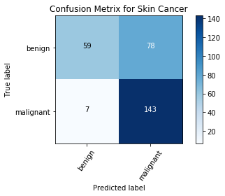
Plotting the Confusion Matrix

Confusion Matrix is a very important metric when analyzing misclassification. Each row of the matrix represents the instances in a predicted class while each column represents the instances in an actual class. The diagonals represent the classes that have been correctly classified. This helps as we not only know which classes are being misclassified but also what they are being misclassified as.



  from sklearn.metrics import classification_report
  classification_report( np.argmax(Y_test, axis=1), np.argmax(Y_pred_tta, axis=1))

  from sklearn.metrics import confusion_matrix

  def plot_confusion_matrix(cm, classes,
                            normalize=False,
                            title='Confusion matrix',
                            cmap=plt.cm.Blues):
      if normalize:
          cm = cm.astype('float') / cm.sum(axis=1)[:, np.newaxis]
          print("Normalized confusion matrix")
      else:
          print('Confusion matrix, without normalization')

      print(cm)

      plt.imshow(cm, interpolation='nearest', cmap=cmap)
      plt.title(title)
      plt.colorbar()
      tick_marks = np.arange(len(classes))
      plt.xticks(tick_marks, classes, rotation=55)
      plt.yticks(tick_marks, classes)
      fmt = '.2f' if normalize else 'd'
      thresh = cm.max() / 2.
      for i, j in itertools.product(range(cm.shape[0]), range(cm.shape[1])):
          plt.text(j, i, format(cm[i, j], fmt),
                   horizontalalignment="center",
                   color="white" if cm[i, j] > thresh else "black")

      plt.ylabel('True label')
      plt.xlabel('Predicted label')
      plt.tight_layout()

  cm = confusion_matrix(np.argmax(Y_test, axis=1), np.argmax(Y_pred, axis=1))

  cm_plot_label =['benign', 'malignant']
  plot_confusion_matrix(cm, cm_plot_label, title ='Confusion Metrix breast cancer classification')

cnfmtrx

Saving the model to disk for reuse

Now, the trained model needs to be serialized. The architecture or structure of the model will be stored in a json file and the weights will be stored in hdf5 file format.



#Save the model
# serialize model to JSON
model_digit_json = model.to_json()
with open("model_digit.json", "w") as json_file:
    json_file.write(model_digit_json)
# serialize weights to HDF5
model.save_weights("model_digit.h5")
print("Saved model to disk")

Hence the saved model can be reused later or easily ported to other environments too.

References

Liu, K., Kang, G., Zhang, N., & Hou, B. (2018). Breast cancer classification based on fully-connected layer first convolutional neural networks. IEEE Access, 6, 23722-23732.
Wang, Z., Li, M., Wang, H., Jiang, H., Yao, Y., Zhang, H., & Xin, J. (2019). Breast cancer detection using extreme learning machine based on feature fusion with CNN deep features. IEEE Access, 7, 105146-105158.