Knowledge Graphs

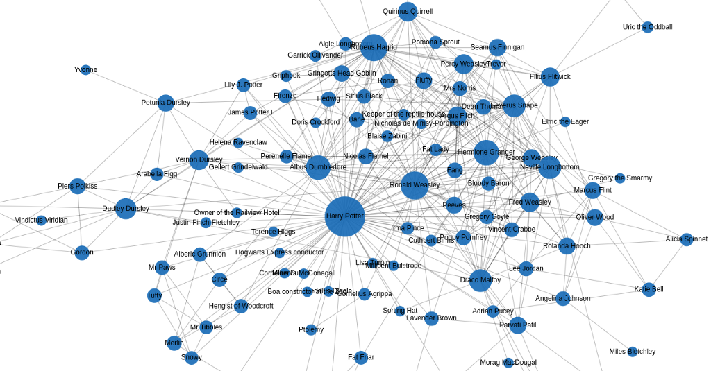
Knowledge Graphs (KGs) have emerged as a compelling abstraction for organizing the world’s structured knowledge, and as a way to integrate information extracted from multiple data sources. Knowledge graphs have started to play a central role in representing the information extracted using natural language processing and computer vision. Domain knowledge expressed in KGs is being input into machine learning models to produce better predictions.

The objecties of this blog post are as follows:

• Explain the basic terminology, concepts, and usage of KGs.
• Highlight recent applications of KGs that have led to a surge in their popularity
• How KGs has placed themselves in the overall landscape of AI.

What are Knowledge Graphs?

A directed labeled graph is a 4-tuple G = (N, E, L, f), where N is a set of nodes, E ⊆ N × N is a set of edges, L is a set of labels, and f: E→L, is an assignment function from edges to labels. An assignment of a label B to an edge E=(A,C) can be viewed as a triple (A, B, C) and visualized as shown in Figure 1.

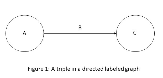
A knowledge graph is a directed labeled graph in which we have associated domain specific meanings with nodes and edges. Anything can act as a node, for example, people, company, computer, etc. An edge label captures the relationship of interest between the nodes, for example, a friendship relationship between two people, a customer relationship between a company and person, or a network connection between two computers, etc.

The directed labeled graph representation is used in a variety of ways depending on the needs of an application. A directed labeled graph such as the one in which the nodes are people, and the edges capture the parent relationship is also known as a data graph. A directed labeled graph in which the nodes are classes of objects (e.g., Book, Textbook, etc.), and the edges capture the subclass relationship, is also known as a taxonomy. In some data models, given a triple (A,B,C), we refer to A, B, C as the subject, the predicate, and the object of the triple respectively.

A knowledge graph serves as a data structure in which an application stores information. The information could be added to the knowledge graph through a combination of human input, automated and semi-automated methods. Regardless of the method of knowledge entry, it is expected that the recorded information can be easily understood and verified by humans.

Many interesting computations over a graph can be reduced to navigating it. For example, in a friendship KG, to calculate the friends of friends of a person A, we can navigate the graph from A to all nodes B connected to it by a relation labeled as friend, and then recursively to all nodes C connected by the friend relation to each B.

Applications of Knowledge Graphs

Use of directed labeled graphs as a data structure for storing information, and the use of graph algorithms to manipulate that information is not new. Within computer science, there have been many uses of a directed graph representation, for example, data flow graphs, binary decision diagrams, state charts, etc. We consider here two concrete applications that have led to a recent surge in the popularity of knowledge graphs: organizing information over the internet and data integration in enterprises. While discussing these applications, we also highlight what is new and different in the use of knowledge graphs.

Organizing Knowledge over the Internet

Consider the Google search for “Winterthur Zurich” which returns the result shown in the left panel of Figure 2 and a relevant portion from Wikipedia in the panel on the right. The portion of the Wikipedia page shown in the panel on the right is also known as an Infobox.

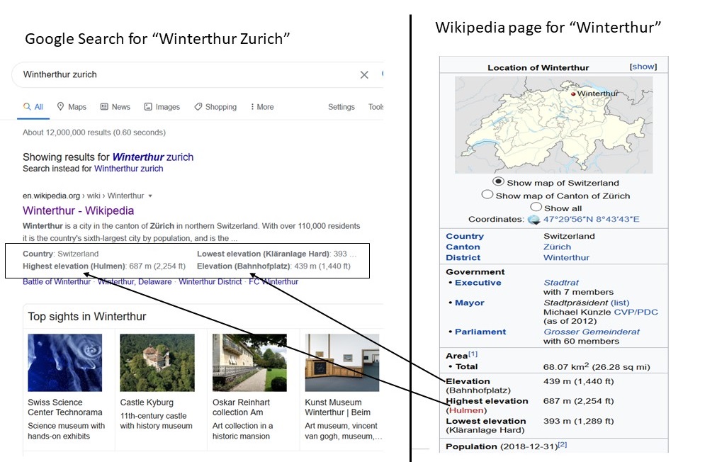
Figure 2: An example use of a knowledge graph in the results of a web search

As part of the search results, we see facts such as Winterthur is in the country Switzerland, its elevation is 430 meters, etc. This information is directly extracted from the Infoboxes from the Wikipedia page for Winterthur. Some of the data in the Wikipedia Infoboxes is populated by querying a KG called Wikidata. The data from a KG can enhance the web search in even deeper ways than illustrated in the above example, as we next discuss.

The Wikipedia page for Winterthur lists its twin towns: two are in Switzerland, one in Czech Republic, and one in Austria. The city of Ontario in California that has a Wikipedia page titled, Ontario, California, lists Winterthur as its sister city. Sister city and twin city relationships are identical as well as reciprocal. Thus, if a city A is a sister (twin) city of another city B, then B must be a sister (twin) city of A. As “Sister cities” and “Twin towns” are section headings in Wikipedia, with no definition or relationship specified between the two, it is difficult to detect this discrepancy.

In contrast, in the Wikidata representation of Winterthur, there is a relationship called twinned administrative body that lists the city of Ontario. As this relationship is defined to be a symmetric relationship in the KG, the Wikidata page for the city of Ontario automatically includes Winterthur. Wikidata solves the problem of identifying equivalent relationships through the effort of its curators, and by using a KG as a storage and inference mechanism. To the degree the Wikidata KG is fully integrated into Wikipedia, the discrepancies of missing links considered in the example considered here will naturally disappear. We can visualize the two way relationship between Winterthur and Ontario in Figure 3. The KG in Figure 3 also shows other objects to which Winterthur and Ontario are connected.

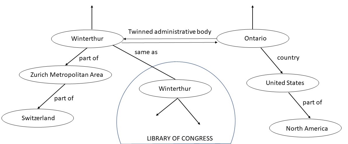
Figure 3: A fragment of the Wikidata knowledge graph

Wikidata includes data from several independent providers such as the Library of Congress. By using the Wikidata identifier for Winterthur, the information released by the Library of Congress can be easily linked with other information about Winterthur present in Wikidata. Wikidata makes it easy to establish such links by publishing the definitions of relationships used in it in Schema.Org.

A well-documented list of relations in Schema.Org, also known as the relation vocabulary, gives us, at least, two advantages. First, it is easier to write queries that span across multiple datasets because queries can be framed using relations that are common to those sources. Without the usage of such common relationships across multiple sources, we would need to determine semantic relationships between them and provide appropriate translations.

One example of a query that goes across multiple sources is: Display on a map the birth cities of people who died in Winterthour? Second, search engines can use such queries to retrieve information from the KG and display the query results as shown in Figure 2. Use of structured information returned in the search results is now a standard feature for the leading search engines.

A recent version of Wikidata had over 90 million objects, with over one billion relationships among those objects. Wikidata makes connections across over 4872 different catalogs in 414 different languages published by independent data providers. As per a recent estimate, 31% of the websites, and over 12 million data providers are currently using the vocabulary of Schema.Org to publish annotations to their web pages.

What is particularly new and exciting about the Wikidata knowledge graph? First, it is a graph of unprecedented scale, and is one of the largest knowledge graphs available today. Second, even though Wikidata is manually curated, the cost of curation is shared by a community of contributors. Third, some of the data in Wikidata may come from automatically extracted information, but it must be easily understood and verified as per the Wikidata editorial policies. Fourth, there is an explicit effort to provide semantic definitions of different relation names through the vocabulary in Schema.Org. Finally, the primary driving use case for Wikidata is to improve the web search. Even though Wikidata has several applications using it for analysis and visualization, its use over the web continues to be the most compelling and easily understood application.

Data Integration in Enterprises

Figure 4: 360-degree view of a customer is created by integrating external data with internal company information

Many financial institutions are interested in better managing their customer relationships through a 360-degree view, i.e., a view that integrates external information about a customer with internal information about the same customer. For example, one can integrate publicly available information from financial news, commercially sourced and curated data about supply chain relationships with internal customer information to create such a 360-degree view.

To understand how such a view is useful, let us consider an example scenario. Financial news reports that “Acma Retail Inc’’ has filed for bankruptcy due to the pandemic, because of which many of its suppliers will face financial stress. Such stress can pass deep down into its supply chain and trigger financial difficulties for other clients.

For example, if a company A who is a supplier for Acma is undergoing financial stress, a similar stress will be experienced by companies who are suppliers of A. Such supply chain relationships are curated as part of a commercially available dataset called Factset. In a 360-degree view, the data from Factset and the financial news are integrated with the internal customer databases. The resulting KG accurately tracks Acma supply chain, identifies stressed suppliers with different revenue exposure, and identifies companies whose risk may be worth monitoring.

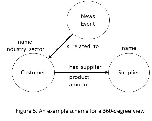
To create the 360-degree view of a customer, the data integration process begins with business analysts sketching out a schema of the key entities, events and the relationships they are interested in tracking. The visual nature of the KG schemas makes it easier for the business experts to engage and specify their requirements.

The data from the individual sources is then loaded into a knowledge graph engine. The storage format of triples allows us to translate only those relationships that are of immediate relevance to the schema defined by the business domain experts. Rest of the data can still be loaded as triples but does not require us to incur the upfront cost of relating them into the defined schema. As the KGs use a generic schema of triples, changing requirements during the analysis process are easier to incorporate. Finally, the storage format mirrors the schema that the domain experts define.

What is particularly new and exciting about the use of knowledge graphs for data integration? First, a generic schema of triples substantially reduces the cost of starting with a data integration project. Second, it is much easier to adapt a triple-based schema in response to changes than the comparable effort required to adapt a traditional relational database. Third, and finally, modern KG engines are highly optimized for answering questions that require traversing the graph relationships in the data.

For the example schema of Figure 5, a graph engine has built in operations to identify the central suppliers in a supply chain network, closely related groups of customers or suppliers, and spheres of influence of different suppliers. All of these computations leverage domain-independent graph algorithms such as centrality detection and community detection. Because of ease of creating and visualizing the schema, and the built in analytics operations, KGs are becoming a popular solution for turning data into intelligence.

Knowledge Graphs in Artificial Intelligence

AI agents maintain representations of the real world and use them for reasoning. Coming up with a good representation is a problem central to AI as it allows an agent to store information and derive new conclusions from it. We begin this section by a quick review of the previous work on knowledge representation in AI, situate KGs within that context, and then provide more details about how the modern AI algorithms use KGs to store their output as well as consume them to incorporate domain knowledge.

Knowledge graphs, also known as semantic networks in the context of AI, have been used as a store of world knowledge for AI agents since the early days of the field, and have been applied in all areas of computer science. There are many other schemes that parallel semantic networks, such as conceptual graphs, description logics, and rule languages. In some cases, probabilistic graphical models can capture uncertain knowledge.

A widely known application of approaches that originated from semantic networks is in capturing ontologies. An ontology is a formal specification of the relationships that are used in a knowledge graph. For example, in Figure 3, the concepts such as City, Country, etc. and relationships such as part of, same as, etc, and their formal definitions constitute an ontology. Using this ontology, we can draw inferences such as Winterthur is located in Switzerland.

To make the internet more intelligent, the World Wide Web Consortium (W3C) standardized a family of knowledge representation languages that are now widely used for capturing knowledge on the internet. These languages include the Resource Description Framework (RDF), the Web Ontology Language(OWL), and the Semantic Web Rule Language (SWRL).

The prior work on knowledge representation in AI that we have just reviewed has been driven in a top-down manner, that is, we first develop a model of the world, and then use reasoning algorithms to draw conclusions from them. Currently, there is a surge of activity on bottom up approaches to AI, that is, developing algorithms that can process the data from which algorithms can draw conclusions and insights. For the rest of the section, we will discuss the role KGs are playing both in storing the learned knowledge, and in providing a source of domain knowledge input to the AI algorithms.

Knowledge Graphs as the output of Machine Learning

Even though Wikidata has had success in engaging a community of volunteer curators, manual creation of knowledge graphs is, in general, expensive. Therefore, any automation we can achieve for creating a knowledge graph is highly desired. Until a few years ago, both natural language processing (NLP) and computer vision (CV) algorithms were struggling to do well on entity recognition from text and object detection from images. Because of recent progress, these algorithms are starting to move beyond the basic recognition tasks to extracting relationships among objects necessitating a representation in which the extracted relations could be stored for further processing and reasoning. We will now discuss how the automation possible through NLP and CV techniques is facilitating the creation of knowledge graphs.

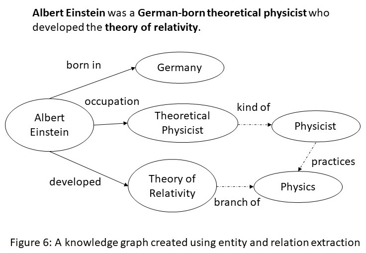
Entity extraction and relation extraction from text are two fundamental tasks in NLP. Methods for performing entity and relation extraction include rule-based methods, and machine learning. The rule-based approaches leverage the syntactical structure of the sentence or specify how entities or relationships could be identified in the input text. The machine learning approaches leverage sequence labeling algorithms or language models for both entity and relation extraction.

The extracted information from multiple portions of the text needs to be correlated, and knowledge graphs provide a natural medium to accomplish such a goal. For example, from the sentence shown in Figure 6, we can extract the entities Albert Einstein, Germany, Theoretical Physicist, and Theory of Relativity; and the relations born in, occupation and developed. Once this snippet of knowledge is incorporated into a larger KG, we can use logical inference to get additional links (shown by dotted edges) such as a Theoretical Physicist is a kind of Physicist who practices Physics, and that Theory of Relativity is a branch of Physics.

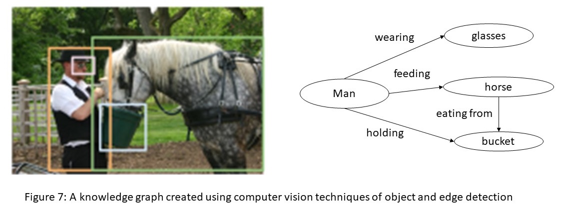
A holy grail of computer vision is the complete understanding of an image, that is, detecting objects, describing their attributes, and recognizing their relationships. Understanding images would enable important applications such as image search, question answering, and robotic interactions. Much progress has been made in recent years towards this goal, including image classification and object detection. Computer vision algorithms make heavy use of machine learning methods such as classification, clustering, nearest neighbors, and the deep learning methods such as recurrent neural networks.

From the image shown in Figure 7, an image understanding system should produce a KG shown to the right. The nodes in the knowledge graph are the outputs of an object detector. Current research in computer vision focuses on developing techniques that can correctly infer the relationships between the objects, such as, man holding a bucket, and horse feeding from the bucket, etc. The KG shown to the right is an example of a knowledge graph which provides foundation for visual question answering.

Knowledge Graphs as input to Machine Learning

Machine learning algorithms can perform better if they can incorporate domain knowledge. KGs are a useful data structure for capturing domain knowledge, but machine learning algorithms require that any symbolic or discrete structure, such as a graph, should first be converted into a numerical form. We can convert symbolic inputs into a numerical form using a technique known as embeddings. To illustrate this, we will consider word embeddings and graph embeddings.

Word embeddings were originally developed for calculating similarity between words. To understand the word embeddings, we consider the following set of sentences.

- I like knowledge graphs.
- I like databases.
- I enjoy running.

In the above set of sentences, we count how often a word appears next to another word and record the counts in a matrix. For example, the word I appears next to the word like twice, and next to the word enjoy once, and therefore, its counts for these two words are 2 and 1 respectively, and 0 for every other word. We can calculate the counts for the other words in a similar manner as shown in Table 1. Such a matrix is often referred to as word co-occurrence counts.

The meaning of each word is captured by the vector in the row corresponding to that word. To calculate similarity between words, we calculate the similarity between the vectors corresponding to them. In practice, we are interested in text that may contain millions of words, and a more compact representation is desired. As the co-occurrence matrix is sparse, we can use techniques from Linear Algebra (e.g., singular value decomposition) to reduce its dimensions. The resulting vector corresponding to a word is known as its word embedding. Typical word embeddings in use today rely on vectors of length 200.

counts	I	like	enjoy	Knowledge	graphs	database	running	.
I	0	2	1	0	0	0	0	0
like	2	0	0	1	0	1	0	0
enjoy	1	0	0	0	0	0	1	0
knowledge	0	1	0	0	1	0	0	0
graphs	0	0	0	1	0	0	0	1
databases	0	1	0	0	0	0	0	1
running	0	0	1	0	0	0	0	1
.	0	0	0	0	1	1	1	0

Table 1: Matrix of co-occurrence counts

A sentence is a sequence of words, and word embeddings calculate co-occurrences of words in it. We can generalize this idea to node embeddings for a graph in the following manner:

(a) traverse the graph using a random walk giving us a path through the graph (b) obtain a set of paths through repeated traversals of the graph (c) calculate co-occurrences of nodes on these paths just like we calculated co-occurrences of words in a sentence (d) each row in the matrix of co-occurrence counts give us a vector for the node corresponding to it (e) use suitable dimensionality reduction techniques to obtain a smaller vector which is referred to as a node embedding.

We can encode the whole graph into a vector which is known as its graph embedding. There are many approaches to calculate graph embeddings, but perhaps, the simplest approach is to add the vectors representing node embeddings for each of the nodes in the graph to obtain a vector representing the whole graph.

We used the example of word embeddings as precursor to explaining graph embeddings primarily for pedagogical purposes. Indeed, both have similar objectives: while word embeddings capture the meaning of words and help calculate similarity between them, node embeddings capture the meaning of nodes in a graph and help calculate similarity between them. There is also a great deal of similarity between the methods used for calculating them.

Word embeddings and graph embeddings are a way to give a symbolic input to a machine learning algorithm. A common application of word embeddings is to learn a language model that can predict what word is likely to appear next in a sequence of words. A more advanced application of word embeddings is to use them with a KG – for example, the embedding for a more frequent word could be reused for a less frequent word as long as the knowledge graph encodes that the less frequent word is its hyponym.

A straightforward use for the graph embeddings calculated from a friendship graph is to recommend new friends. A more advanced use of graph embedding involves link prediction, for example, in a company graph, we can use link prediction to identify potential new customers.

Conclusions

A directed labeled graph is a fundamental construct in discrete mathematics, and has applications in all areas of computer science. Most notable uses of directed labeled graphs in AI and databases have taken the form of data graphs, taxonomies and ontologies. Traditionally, such applications have been small and have been created by a top down design and through manual knowledge engineering.

Distinguishing characteristics of the modern knowledge graphs from the classical knowledge graphs are: scale, bottom up development and multiple modes of construction. The early semantic networks in AI never reached the size and scale of the knowledge graphs that we see today. Difficulty in coming up with a top down schema design for data integration and the data driven nature of machine learning have forced a bottom up methodology for creating the knowledge graphs. Finally, for creating modern knowledge graphs we are supplementing manual knowledge engineering techniques with significant automation and crowdsourcing

References

• Hogan, Aidan, et al. "Knowledge graphs." ACM Computing Surveys (CSUR) 54.4 (2021): 1-37.
• Bellomarini, Luigi, et al. "Knowledge graphs and enterprise AI: the promise of an enabling technology." 2019 IEEE 35th International Conference on Data Engineering (ICDE). IEEE, 2019.