Principal Component Analysis (PCA)

Principal component analysis (PCA) in its typical form implicitly assumes that the observed data matrix follows a Gaussian distribution. However, PCA can be generalized to allow for other distributions – here, we take a look at its generalization for exponential families introduced by Collins et al. in 2001.

The exponential family

The exponential family of distributions plays a major role in statistical theory and practical modeling. A large reason for this is that the family allows for many nice closed-form results and asymptotic guarantees for performing estimation and inference. Additionally, the family is fairly diverse and can model lots of different types of data.

Recall the basic form of an exponential family density (here, using Wikipedia’s notation):

Here, $T(x)$ is a sufficient statistic, $\eta(\theta)$ is the “natural parameter”, $A(\theta)$ is a normalizing factor that makes the distribution sum to $1$, and $h(x)$ is the base measure. The form of $A(\theta)$ is determined automatically once the other functions have been determined. Its form can perhaps more easily seen by writing

Thus, enforcing $f$ sum to $1$, we must have that

Rearranging, we have

or, equivalently,

In canonical form, we have $\eta(\theta) = \theta$, and it is also often the case that $T(x) = x$. In this case, the form simplifies to

Thus, by expanding $A$, we can see that $f$ can also be written as

An important property of $A(\theta)$ is that its first derivative with respect to $\theta$ is equal to the expectation of $f$:

\begin{align} A’(\theta) &= \sum\limits_{x \in \mathcal{X}} x \frac{h(x) \exp\left\{ \theta x \right\}} {\sum\limits_{x \in \mathcal{X}} h(x) \exp\left\{ \theta x \right\}} \\ &= \sum\limits_{x \in \mathcal{X}} x f(x | \theta) \\ &= \mathbb{E}_{f(x)}[x | \theta] \end{align}

Generalized linear models

In the setting of (generalized) linear models, we have a design matrix $\mathbf{X} \in \mathbb{R}^{n \times p}$ and a vector of response variables $\mathbf{Y} \in \mathbb{R}^n$, and we’re interested in in finding a linear relationship between them. Often we assume that the conditional density of $\mathbf{Y} | \mathbf{X}$ is in the exponential family.

Modeling a linear relationship directly as $\mathbb{E}[\mathbf{Y} | \mathbf{X}] = \mathbf{X} \boldsymbol{\beta}$ for a parameter vector $\boldsymbol{\beta} \in \mathbb{R}^p$ implicitly assumes Gaussian errors when a mean-squared error loss is used. However, to accommodate non-Gaussian distributions, we can transform the expected value with a “link function” $g$. Denote $\mu(x) = \mathbb{E}[\mathbf{Y} | \mathbf{X}]$. Then we say

Recall that $A’(\theta) = \mu(x)$, so we have

\begin{align} &\mu(x) = g^{-1}(\mathbf{X} \boldsymbol{\beta}) = A’(\theta) \\ \implies &\theta = (A’ \circ g)^{-1}(\mathbf{X} \boldsymbol{\beta}) \end{align}

where $\circ$ denotes a composition of the two functions.

A “canonical” link function is defined as $g = (A’)^{-1}$, and in this case we have $\theta = (A’ \circ (A’)^{-1})^{-1}(\mathbf{X} \boldsymbol{\beta}) = \mathbf{X} \boldsymbol{\beta}$.

For simplicity (and practical relevance), the rest of this post assumes the use of a canonical link function. To fit a GLM, we can write down the likelihood of the parameters $\boldsymbol{\beta}$ given the data $\mathbf{X}, \mathbf{Y}$, and maximize that likelihood using standard optimization methods (gradient descent, Newton’s method, Fisher scoring, etc.). The likelihood for a sample $Y_1, \dots, Y_n$ and $X_1, \dots, X_n$ looks like:

\begin{align} L &= \prod\limits_{i=1}^n h(Y_i) \exp\left\{ \theta Y_i - A(\theta) \right\} \\ &= \prod\limits_{i=1}^n h(Y_i) \exp\left\{ X_i \beta Y_i - A(X_i \beta) \right\} \\ \end{align}

The log-likelihood is

We can then maximize this with respect to $\beta$, which effectively amounts to maximizing $\sum\limits_{i=1}^n \left[ X_i \beta Y_i - A(X_i \beta) \right]$ because the term $\log h(Y_i)$ is constant with respect to $\beta$.

From GLMs to PCA

Now, suppose we have a data matrix $\mathbf{X} \in \mathbb{R}^{n \times p}$, and instead of finding a relationship with some response vector, we’d like to understand the patterns of variation within $\mathbf{X}$ alone. We can use a similar modeling approach as that of GLMs (where we assume a linear relationships), but now we model $\mathbb{E}[\mathbf{X}] = \mathbf{A}\mathbf{V}$, where $\mathbf{A}$ and $\mathbf{V}$ are two lower-rank matrices ($\mathbf{A} \in \mathbb{R}^{n \times k}$, and $\mathbf{V} \in \mathbb{R}^{k \times p}$, where $k < p$), neither of which is observed. Notice that now both our “design matrix” and our parameter vector are unknown, unlike in the case of GLMs where we observed a design matrix.

This is precisely the approach taken in a paper by Collins et al. called “A Generalization of Principal Component Analysis to the Exponential Family”. The rest of this post explores the details of this paper.

To be more precise, let $\Theta \in \mathbb{R}^{n \times p}$ be a matrix of canonical parameters. We are now trying to find $\mathbf{A}$ and $\mathbf{V}$ to make the approximation

where $\mathbf{A} \in \mathbb{R}^{n \times k}$ and $\mathbf{V} \in \mathbb{R}^{k \times p}$. Assume $k=1$ for now, again for simplicity. In this case, $\mathbf{A}$ and $\mathbf{V}$ are vectors, so let’s denote them as $\mathbf{a}$ and $\mathbf{v}$. Using the exponential family form above, the likelihood is then

\begin{align} \log L(\mathbf{a}, \mathbf{v}) &= \sum\limits_{i = 1}^n \sum\limits_{j = 1}^p \left(\theta_{ij} x_{ij} - A(\theta_{ij}) \right) \\ &= \sum\limits_{i = 1}^n \sum\limits_{j = 1}^p \left( a_i v_j x_{ij} - A(a_i v_j) \right) \\ \end{align}

where $a_i$ is the $i$th element of $\mathbf{a}$, and $v_j$ is the $j$th element of $\mathbf{v}$.

Now we can maximize this likelihood with respect to $\mathbf{A}$ and $\mathbf{V}$. A common way to do this is via alternating minimization of the negative log-likelihood (which is equivalent to maximizing the log-likelihood), which proceeds as:

1. Fix $\mathbf{v}$, and minimize the negative log-likelihood w.r.t. $\mathbf{a}$.
2. Fix $\mathbf{a}$, and minimize the negative log-likelihood w.r.t. $\mathbf{v}$.
3. Repeat Steps 1-2 until convergence.

It turns out that these minimization problems are convex in $\mathbf{a}$ and $\mathbf{v}$ individually (while the other one is held fixed), but not convex in both $\mathbf{a}$ and $\mathbf{v}$ simultaneously.

One way to view this problem is as $n + p$ GLM regression problems, where each regression problem has one parameter. For example, when fitting the $i$th element of $\mathbf{a}$, $a_i$ while $\mathbf{v}$ is fixed, we have the following approximation problem:

where $\Theta_i$ is the $i$th row of $\Theta$.

This leads to the following log-likelihood:

where the subscript $j$ indicates the $j$th element of a vector.

We can see a correspondence to the typical univariate GLM setting in which we have observed data:

\begin{align} a_i &\iff \boldsymbol{\beta}\; \text{(parameter)} \\ \mathbf{v} &\iff \mathbf{X} \; \text{(Design matrix)} \\ \mathbf{X}_i &\iff \mathbf{Y} \; \text{(Response vector)} \end{align}

where $\mathbf{X}_i \in \mathbb{R}^p$ is the $i$th row of $\mathbf{X}$. A similar correspondence exists when we fit $\mathbf{v}_j$ while holding $\mathbf{A}$ fixed.

Examples

Gaussian (PCA)

If we assume Gaussian observations with fixed unit variance, then the only parameter is the mean $\mu$. In this case have $A(\theta) = \frac{1}{2} \theta^2 = \frac12 \mu^2$. We also have $A’(\theta) = \mu$, which is indeed the expected value. The log-likelihood of the PCA model is

Minimizing the negative log-likelihood is also equivalent to minimizing the mean-squared error:

Again, realizing that that this problem decomposes into $n + p$ regression problems, we can solve for the updates for $\mathbf{a}$ and $\mathbf{v}$. The minimization problem for $a_i$ is

\begin{align} \min_{a_i} \sum\limits_{j=1}^p \left[ -a_i v_j x_{ij} + \frac12 (a_i v_j)^2 \right] \end{align}

In vector form for $\mathbf{a}$, we have

\begin{align} \min_{\mathbf{a}} \frac12 ||\mathbf{X} - \mathbf{V} \mathbf{a}^\top||_2^2 \end{align}

Of course, this has the typical least squares solution. Here’s a quick derivation for completeness:

Equating this gradient to 0, we have

\begin{align} &\mathbf{v}^\top \mathbf{X} - \mathbf{v}^\top \mathbf{v} \mathbf{a} = 0 \\ \implies& \mathbf{a} = (\mathbf{v}^\top \mathbf{v})^{-1} \mathbf{v}^\top \mathbf{X} \end{align}

Since $\mathbf{v}$ is a vector, this simplifies to

Similarly, the update for $\mathbf{v}$ is

So the alternating least squares algorithm for Gaussian PCA is

1. Update $\mathbf{a}$ as $\mathbf{a} = \frac{\mathbf{v}^\top \mathbf{X}_i}{||\mathbf{v}||_2^2}$.
2. Update $\mathbf{v}$ as $\frac{\mathbf{a}^\top \mathbf{X}_i}{||\mathbf{a}||_2^2}$.
3. Repeat Steps 1-2 until convergence.

Of course, the Guassian case is particularly nice in that it has an analytical solution for the minimum each time. This isn’t the case in general – let’s see a (slightly) more complex example below.

Bernoulli

With a Bernoulli likelihood, each individual regression problem now boils down to logistic regression. The normalizing function in this case is $A(\theta) = \log\left\{ 1 + \exp(\theta)\right\}$. Thus, the optimization problem for $\mathbf{a}_i$ is

Of course, there’s no analytical solution in this case, so we can resort to iterative optimization methods. For example, to perform gradient descent, the gradient is

Similarly the gradient for $v_j$ is

Then, for some learning rate $\alpha$, we could run

1. For $i \in [n]$, update $a_i$ as $a_i = a_i - \alpha \nabla_{a_i} \left[- \log L\right]$.
2. For $j \in [p]$, update $v_j$ as $v_j = v_j - \alpha \nabla_{v_j} \left[- \log L\right]$.
3. Repeat Steps 1-2 until convergence.

Simulations

Here’s some simple code for performing alternating least squares with Guassian data as desribed above. Recall that we’re minimizing the negative log-likelihood here, which is equivalent to maximizing the log-likelihood.

import numpy as np
import matplotlib.pyplot as plt

n = 40
p = 2
k = 1

A_true = np.random.normal(size=(n, k))
V_true = np.random.normal(size=(k, p))
X = np.matmul(A_true, V_true) + np.random.normal(size=(n, p))
X -= np.mean(X, axis=0)

num_iters = 100

A = np.random.normal(loc=0, scale=1, size=(n, k))
V = np.random.normal(loc=0, scale=1, size=(k, p))

for iter_num in range(num_iters):
    A = np.matmul(X, V.T) / np.linalg.norm(V, ord=2)**2
    V = np.matmul(A.T, X) / np.linalg.norm(A, ord=2)**2

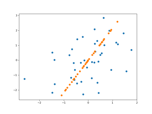
And here’s a plot of the projected data onto the inferred line (here, plotting the “reconstruction” of $\mathbf{X}$ from its inferred components).

Here’s code for doing “logistic PCA”, or PCA with bernoulli data. I used Autograd to easily compute the gradients of the likelihood here.

import matplotlib.pyplot as plt
from autograd import grad
import autograd.numpy as np

n = 100
p = 2
k = 1

A_true = np.random.normal(size=(n, k))
V_true = np.random.normal(size=(k, p))
X_probs = 1 / (1 + np.exp(-np.matmul(A_true, V_true)))
X = np.random.binomial(n=1, p=X_probs)

def bernoulli_link(x):
    return 1 / (1 + np.exp(-x))

def bernoulli_likelihood_A(curr_A):
    return -np.sum(np.log(np.matmul(X.T, X))) - np.sum(np.multiply(np.matmul(curr_A, V), X)) + np.sum(np.log(1 + np.exp(np.matmul(curr_A, V))))

def bernoulli_likelihood_V(curr_V):
    return -np.sum(np.log(np.matmul(X.T, X))) - np.sum(np.multiply(np.matmul(A, curr_V), X)) + np.sum(np.log(1 + np.exp(np.matmul(A, curr_V))))

num_iters = 500

A = np.random.normal(loc=0, scale=1, size=(n, k))
V = np.random.normal(loc=0, scale=1, size=(k, p))

A_grad = grad(bernoulli_likelihood_A)
V_grad = grad(bernoulli_likelihood_V)
learning_rate = 1e-2

for iter_num in range(num_iters):
    curr_grad_A = A_grad(A)
    curr_grad_V = V_grad(V)

    A -= learning_rate * curr_grad_A
    V -= learning_rate * curr_grad_V

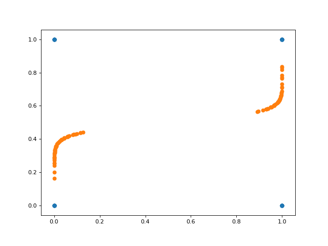
And here’s a plot of the projected data onto the inferred space. Notice in this case that the inferred subspace is nonlinear in the original space.

Conclusions

Here, we walked through a generalized version of PCA that allows us to account for non-Gaussian data.

References

• Collins, Michael, Sanjoy Dasgupta, and Robert E. Schapire. “A generalization of principal components analysis to the exponential family.” Advances in neural information processing systems. 2002.
• Alex Williams’s blog post on logistic PCA