Tanveer Khan Data Scientist @ NextGen Invent | Research Scholar @ Jamia Millia Islamia
Time series based feature extraction: Electrocardiogram (ECG) data
In this article we will examine the times series based feature extraction techniques more specifically, Fourier and Wavelet transforms. We will extract frequency and wavelet features from ECG data to train a classification model.
1. Introduction
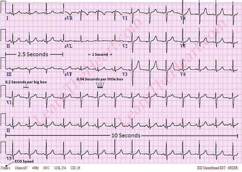
Electrocardiogram (ECG) is a non-invasive technique to record the heart's electrical activity by placing electrodes on the chest. The end product of the ECG is the electrogram which is a graph of voltage versus time of the electrical activity of the heart.
Feature extraction remains an important step in building the classification models. Here, we will extract frequency domain and time-frequency domain features from our ECG data. Frequency features are extracted by applying Fast Fourier Transform (FFT) on our ECG data. To extract time-frequency features we will apply wavelet transform on our time series data.
2. About Dataset
ECG data set consisting of 162 ECG recordings and diagnostic labels. The data are sampled at 128 hertz.
3. Methodology
Typical ECG signal classification pipeline includes tasks such as: signal-acquisition, signal pre-processing, features extraction, and classification phase.
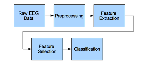
Figure 1. ECG signal processing steps
Here, our ECG data is already acquired and pre-processed so, we can start from the next phase in the pipeline which is the feature extraction phase.
To proceed further to the next phase, first, we have to load the data and then segregate the features and labels values from our ECG data. We will also apply some visualiztions to go through with the ECG data.
4. Building a Classification model
Here, in this section we will write python code for building a classification model. We will start by importing relevant packages, and then loading the data, and so on.
4.1 Importing packages
Here, we have imported the relevant packages for the loading of data, visualization, feature extraction, and classification purpose. Below is the code for the same.
%matplotlib inline
import numpy as np
import pandas as pd
import pywt
import seaborn as sns
import scaleogram as scg
import matplotlib.pyplot as plt
import matplotlib.gridspec as GridSpec
from mat4py import loadmat
from scipy.fftpack import fft
4.2 Data Loading
# Create list of data and labels from dictionary
data = loadmat("../article_fft/data/physionet_ECG_data-master/ECGData/ECGData.mat")

ecg_total = len(data['ECGData']['Data'])
ecg_data = []
ecg_labels = []
for i in range(0, ecg_total):
    ecg_data.append(data['ECGData']['Data'][i])
    ecg_labels.append(data['ECGData']['Labels'][i])

flat_list_ecg_labels = [item for sublist in ecg_labels for item in sublist]
4.3 Data Visualization
Here, we plot the raw ECG signal data. Below is the code for the same.
## Data Visualization

fig = plt.figure(figsize=(12, 6))
grid = plt.GridSpec(3, 1, hspace=0.6)

arr_signal = fig.add_subplot(grid[0, 0])
chg_signal = fig.add_subplot(grid[1, 0])
nsr_signal = fig.add_subplot(grid[2, 0])

arr_signal.plot(range(0, len(data['ECGData']['Data'][33]), 1), ecg_data[33], color = 'blue')
arr_signal.set_xlim(0, 1000)
arr_signal.set_title('ARR Signal')

chg_signal.plot(range(0, len(data['ECGData']['Data'][100]), 1), ecg_data[100], color = 'red')
chg_signal.set_xlim(0, 1000)
chg_signal.set_title('CHG Signal')

nsr_signal.plot(range(0, len(data['ECGData']['Data'][150]), 1), ecg_data[150], color = 'green')
nsr_signal.set_xlim(0, 1000)
nsr_signal.set_title('NSR Signal')
plt.close(fig)
Figure below shows the plot of raw ECG signal values.
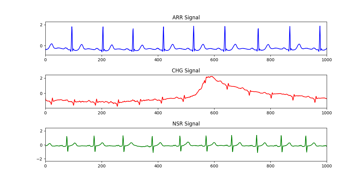
Figure 2. Raw ECG data.
4.4 Feature extraction
From the pre-processed ECG signal data we will extract the frequency and time-frequency domain features. These features are extracted after applying fast fourier (FFT) and wavelet transforms.
Frequency features
#Arr signal Fourier Transform
nn = 160
signal_length = 1000
full_signal_fft_values = np.abs(fft(ecg_data[nn][:signal_length]))
x_values_fft = range(0, len(data['ECGData']['Data'][nn]), 1)[:signal_length]

fig = plt.figure(figsize=(12, 6))
grid = plt.GridSpec(2, 1,hspace=0.6)

full_signal = fig.add_subplot(grid[0, 0])
fft_comp = fig.add_subplot(grid[1, 0])

full_signal.plot(x_values_fft, ecg_data[nn][:signal_length], color = 'green')
full_signal.set_xlim(0, 512)
full_signal.set_title('Full Signal')
fft_comp.plot(x_values_fft, list(full_signal_fft_values), color = 'purple')
fft_comp.set_xlim(0, 512)
fft_comp.set_ylim(0, 100)
fft_comp.set_title('FFT of full signal')
plt.close(fig)
Figure below shows the signal values before and after applying FFT.
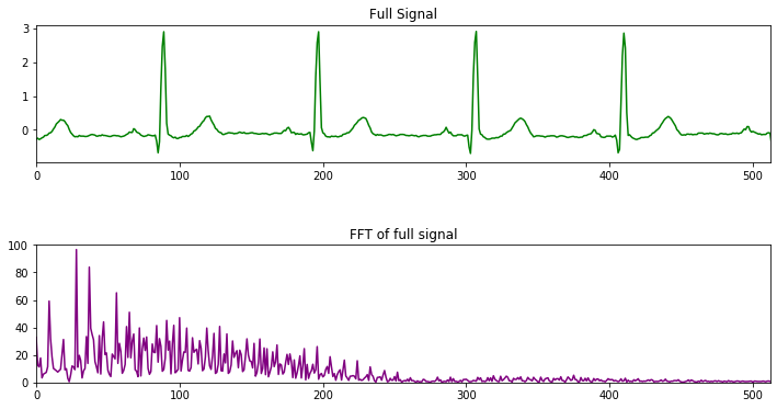
Figure 3. FFT transformed data.
Wavelet features
# choose default wavelet function
scg.set_default_wavelet('morl')

nn = 33
signal_length = 128
# range of scales to perform the transform
scales = scg.periods2scales( np.arange(1, signal_length+1) )
x_values_wvt_arr = range(0,len(ecg_data[nn]),1)

# plot the signal
fig1, ax1 = plt.subplots(1, 1, figsize=(9, 3.5));
ax1.plot(x_values_wvt_arr, ecg_data[nn], linewidth=3, color='blue')
ax1.set_xlim(0, signal_length)
ax1.set_title("ECG ARR")

# the scaleogram
scg.cws(ecg_data[nn][:signal_length], scales=scales, figsize=(10, 4.0), coi = False, ylabel="Period", xlabel="Time",
        title='ECG_ARR: scaleogram with linear period');
print("Default wavelet function used to compute the transform:", scg.get_default_wavelet(), "(",
      pywt.ContinuousWavelet(scg.get_default_wavelet()).family_name, ")")
Figure below shows the signal values before and after applying wavelet transform.
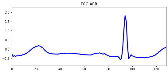
Figure 4. ECG ARR
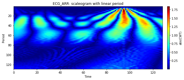
Figure 5. ECG_ARR: scaleogram with linear period
4.5 Classification of ECG data
Here, we will perform the classification of ECG signal data. In this we will build and train a feed forward neural network model for the same.
#Preparing data
arr_list = ecg_data[0:95]
chf_list = ecg_data[96:125]
nsr_list = ecg_data[126:162]

arr_split_256 = [np.array_split(arr_list[ii], 256) for ii in range(95)]
arr_flatten = [item for sublist in arr_split_256 for item in sublist]

chf_split_256 = [np.array_split(chf_list[ii], 256) for ii in range(29)]
chf_flatten = [item for sublist in chf_split_256 for item in sublist]

nsr_split_256 = [np.array_split(nsr_list[ii], 256) for ii in range(36)]
nsr_flatten = [item for sublist in nsr_split_256 for item in sublist]

reduce_size = 500
full_1500 = (arr_flatten[0:reduce_size] + chf_flatten[0:reduce_size] + nsr_flatten[0:reduce_size])

# creating the data set
from sklearn import preprocessing
from sklearn.model_selection import train_test_split

fs = len(full_1500[0])
sgn_length = 2000   #65536   Pay atention with ram memory!
size_dataset = len(full_1500)
scales = range(1, fs)
waveletname = 'morl'

X_full = np.ndarray(shape=(size_dataset, fs-1, fs-1, 3))

for i in range(0, size_dataset):
    if i % 500 == 0:
        print (i, 'done!')
    for j in range(0, 3):
        signal = full_1500[i]
        coeff, freq = pywt.cwt(signal, scales, waveletname, 1)
        X_full[i, :, :, j] = coeff[:,:fs-1]

### Dividing data into training and testing datasets
list_ecg_labels_arr = ['ARR']*reduce_size
list_ecg_labels_chf = ['CHF']*reduce_size
list_ecg_labels_nsr = ['NSR']*reduce_size
list_ecg_labels = (list_ecg_labels_arr + list_ecg_labels_chf + list_ecg_labels_nsr)

le = preprocessing.LabelEncoder()
ecg_labels_encoded = le.fit_transform(list_ecg_labels)
X_train, X_test, y_train, y_test = train_test_split(X_full, ecg_labels_encoded, test_size=0.25, random_state=42)
4.6 Training a NN classifier with ECG Scaleograms
For performing the classification task Feed forward neural network (ANN) is used.
import sys
from tensorflow import keras
#Inspecting DATA
n_rows = 3
n_cols = 5
class_names = ['ARR', 'CHF', 'NSR']
plt.figure(figsize=(n_cols*1.5, n_rows * 1.6))
for row in range(n_rows):
    for col in range(n_cols):
        index = n_cols * row + col
        plt.subplot(n_rows, n_cols, index + 1)
        plt.imshow((X_train[index]*255).astype(np.uint8), cmap="binary", interpolation="spline36")
        plt.axis('off')
        plt.title(class_names[y_train[index]])
plt.show()
Figure below shows an inspection of ECG labels scelogram data.
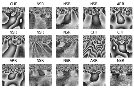
Figure 6. ECG labels scaleogram
Defining the Neural network model architecture.
# Defining basic NN
num_filter, num_classes = 3, 3
model = keras.models.Sequential([
    keras.layers.Flatten(input_shape=[fs-1, fs-1, num_filter]),
    keras.layers.Dense(300, activation="relu"),
    keras.layers.Dense(100, activation="relu"),
    keras.layers.Dense(num_classes, activation="softmax")
])
model.compile(loss="sparse_categorical_crossentropy",
              optimizer="sgd", metrics=["accuracy"])
Figure below shows the model summary.
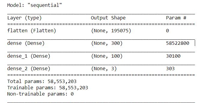
Figure 7. Build NN model summary
Training and evaluation of the NN model.
### Model Training
history = model.fit(X_train, y_train, epochs=10, validation_data=(X_test, y_test))
              optimizer="sgd", metrics=["accuracy"])

## Model evaluation
model.evaluate(X_test, y_test)
Here, we will evaluate the trained NN model perfromance on our test data by calling model.predict() function. We will also plot a confusion matrix as performance measure to find out the actual labels and predicted labels.
# Confusion Matrix With Scikit
from sklearn.metrics import confusion_matrix

cm = confusion_matrix(y_test, pred_classes)
cm_norm =  cm.astype('float') / cm.sum(axis=1)[:, np.newaxis]

# Ploting Confusion Matrix

df_cm = pd.DataFrame(cm_norm, ['ARR', 'CHF', 'NSR'], ['ARR', 'CHF', 'NSR'])
plt.figure(figsize = (10,6))
conf = sns.heatmap(df_cm, annot=True, square=True, annot_kws={"size": 12})
conf.set_xlabel('Prediction')
conf.set_ylabel('True')
Figure below shows the confusion matrix.
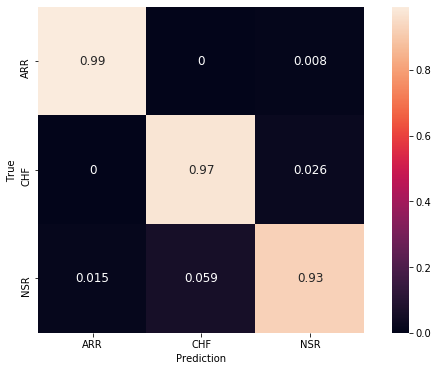
Figure 8. Confusion matrix
4. Conclusion
In this article we have seen two different ways to extact features from signals based on time dependence of frequency distribution, Fourier and Wavelet transforms. These functions transform a signal from the time-domain to the frequency-domain and give us its frequency spectrum.
We have learnt that Fourier transform is the most convenient tool when signal frequencies do not change in time. However, if the frequencies of the signal vary in time the most performant technique is a wavelet transform. Based on ECG data, we made a classification over three groups of people with different pathologies: cardiac arrhythmia, congestive heart failure and healthy people. With a very simple neural network we were able to get a precise model which quickly allows us to detect a healthy person from others with heart disease.
Complete code can be found here.
References
- Ribeiro, A.H., Ribeiro, M.H., Paixão, G.M.M. et al. Automatic diagnosis of the 12-lead ECG using a deep neural network. Nat Commun 11, 1760 (2020).